Total Reads and Mapped Reads (CTCF and RAD21)
Last updated: 2025-10-07
Checks: 7 0
Knit directory: ChIPSeq_project/
This reproducible R Markdown analysis was created with workflowr (version 1.7.1). The Checks tab describes the reproducibility checks that were applied when the results were created. The Past versions tab lists the development history.
Great! Since the R Markdown file has been committed to the Git repository, you know the exact version of the code that produced these results.
Great job! The global environment was empty. Objects defined in the global environment can affect the analysis in your R Markdown file in unknown ways. For reproduciblity it’s best to always run the code in an empty environment.
The command set.seed(20250815) was run prior to running
the code in the R Markdown file. Setting a seed ensures that any results
that rely on randomness, e.g. subsampling or permutations, are
reproducible.
Great job! Recording the operating system, R version, and package versions is critical for reproducibility.
Nice! There were no cached chunks for this analysis, so you can be confident that you successfully produced the results during this run.
Great job! Using relative paths to the files within your workflowr project makes it easier to run your code on other machines.
Great! You are using Git for version control. Tracking code development and connecting the code version to the results is critical for reproducibility.
The results in this page were generated with repository version ffd3efc. See the Past versions tab to see a history of the changes made to the R Markdown and HTML files.
Note that you need to be careful to ensure that all relevant files for
the analysis have been committed to Git prior to generating the results
(you can use wflow_publish or
wflow_git_commit). workflowr only checks the R Markdown
file, but you know if there are other scripts or data files that it
depends on. Below is the status of the Git repository when the results
were generated:
Ignored files:
    Ignored:    .Rhistory
    Ignored:    .Rproj.user/
Note that any generated files, e.g. HTML, png, CSS, etc., are not included in this status report because it is ok for generated content to have uncommitted changes.
These are the previous versions of the repository in which changes were
made to the R Markdown
(analysis/Total_Reads_and_Mapped_Reads_CTCF_RAD21.Rmd) and
HTML (docs/Total_Reads_and_Mapped_Reads_CTCF_RAD21.html)
files. If you’ve configured a remote Git repository (see
?wflow_git_remote), click on the hyperlinks in the table
below to view the files as they were in that past version.
| File | Version | Author | Date | Message |
|---|---|---|---|---|
| Rmd | ffd3efc | sayanpaul01 | 2025-10-07 | Commit |
| html | ffd3efc | sayanpaul01 | 2025-10-07 | Commit |
| Rmd | 4c5ce13 | sayanpaul01 | 2025-08-19 | Commit |
| html | 4c5ce13 | sayanpaul01 | 2025-08-19 | Commit |
| html | 25ce453 | sayanpaul01 | 2025-08-18 | Commit |
| Rmd | ab9a136 | sayanpaul01 | 2025-08-18 | Commit |
| html | ab9a136 | sayanpaul01 | 2025-08-18 | Commit |
| Rmd | 90183c3 | sayanpaul01 | 2025-08-17 | Commit |
| html | 90183c3 | sayanpaul01 | 2025-08-17 | Commit |
| Rmd | 7906757 | sayanpaul01 | 2025-08-15 | Commit |
| html | 7906757 | sayanpaul01 | 2025-08-15 | Commit |
📌 Total Reads by Sample
Load Required Libraries
# Load necessary R packages
library(edgeR)
Warning: package 'edgeR' was built under R version 4.3.2Loading required package: limmaWarning: package 'limma' was built under R version 4.3.1library(limma)
library(RColorBrewer)
library(gridExtra)
library(reshape2)
library(data.table)Warning: package 'data.table' was built under R version 4.3.3
Attaching package: 'data.table'The following objects are masked from 'package:reshape2':
dcast, meltlibrary(tidyverse)Warning: package 'tidyverse' was built under R version 4.3.2Warning: package 'tidyr' was built under R version 4.3.3Warning: package 'readr' was built under R version 4.3.3Warning: package 'purrr' was built under R version 4.3.3Warning: package 'dplyr' was built under R version 4.3.2Warning: package 'stringr' was built under R version 4.3.2Warning: package 'lubridate' was built under R version 4.3.3── Attaching core tidyverse packages ──────────────────────── tidyverse 2.0.0 ──
✔ dplyr 1.1.4 ✔ readr 2.1.5
✔ forcats 1.0.0 ✔ stringr 1.5.1
✔ ggplot2 3.5.2 ✔ tibble 3.2.1
✔ lubridate 1.9.4 ✔ tidyr 1.3.1
✔ purrr 1.0.4 ── Conflicts ────────────────────────────────────────── tidyverse_conflicts() ──
✖ dplyr::between() masks data.table::between()
✖ dplyr::combine() masks gridExtra::combine()
✖ dplyr::filter() masks stats::filter()
✖ dplyr::first() masks data.table::first()
✖ lubridate::hour() masks data.table::hour()
✖ lubridate::isoweek() masks data.table::isoweek()
✖ dplyr::lag() masks stats::lag()
✖ dplyr::last() masks data.table::last()
✖ lubridate::mday() masks data.table::mday()
✖ lubridate::minute() masks data.table::minute()
✖ lubridate::month() masks data.table::month()
✖ lubridate::quarter() masks data.table::quarter()
✖ lubridate::second() masks data.table::second()
✖ purrr::transpose() masks data.table::transpose()
✖ lubridate::wday() masks data.table::wday()
✖ lubridate::week() masks data.table::week()
✖ lubridate::yday() masks data.table::yday()
✖ lubridate::year() masks data.table::year()
ℹ Use the conflicted package (<http://conflicted.r-lib.org/>) to force all conflicts to become errorslibrary(scales)Warning: package 'scales' was built under R version 4.3.2
Attaching package: 'scales'

The following object is masked from 'package:purrr':

    discard

The following object is masked from 'package:readr':

col_factorlibrary(biomaRt)Warning: package 'biomaRt' was built under R version 4.3.2library(cowplot)Warning: package 'cowplot' was built under R version 4.3.2
Attaching package: 'cowplot'

The following object is masked from 'package:lubridate':

stamplibrary(ggrepel)Warning: package 'ggrepel' was built under R version 4.3.3library(corrplot)Warning: package 'corrplot' was built under R version 4.3.3corrplot 0.95 loadedlibrary(Hmisc)Warning: package 'Hmisc' was built under R version 4.3.3
Attaching package: 'Hmisc'

The following objects are masked from 'package:dplyr':

    src, summarize

The following objects are masked from 'package:base':

format.pval, unitslibrary(ggpubr)Warning: package 'ggpubr' was built under R version 4.3.1
Attaching package: 'ggpubr'

The following object is masked from 'package:cowplot':

    get_legend
📍 2. Load Data
align<-read.csv("data/ChIP Seq Summary stat CTCF RAD21.csv")

map<-data.frame(align)

map$Treatment<- factor(map$Treatment, levels = c("VEH_CTCF", "DOX_CTCF", "VEH_RAD21", "DOX_RAD21", "VEH_Input_P53", "DOX_Input_P53"))
📍 3. Define Color Palettes
drug_palc <- c("#8B006D","#DF707E","#F1B72B", "#3386DD","#707031","#41B333")

Ind_palc <- c("#ffbe0b","#ff006e","#fb5607", "#8338ec","#3a86ff","#4a4e69")

Treat_palc <- c("#ffbe0b","#ff006e","#fb5607", "#8338ec", "#800080","#FFC0CB")

Map_palc <- c("#9b19f5","#e6d800", "#b3d4ff")

Combined_palc <- c("#FF0000","#00FF00","#0000FF","#FFFF00","#FF00FF","#00FFFF","#FFA500","#800080","#FFC0CB","#A52A2A","#808080","#FFD700")

Type_palc <- c("#800080","#FFD700")
📍 4. Prepare Data
# Factor Sample_name to maintain order
map$Sample.Det<-factor(map$Sample.Det,levels = map$Sample.Det)
📍 5. Plot Total Reads by Sample
map %>%
  #mutate(Drug=factor(Drug,levels=c("CX-5461","DOX","VEH"))) %>%
  #mutate(Conc.=factor(Conc.,levels=c("0.1","0.5"))) %>%
  #mutate(Time=factor(Time,levels=c("3","24","48"))) %>%
  #group_by(Drug,Conc.,Time) %>%
  ggplot(., aes (x =Sample.Det, y=Total.Reads..before.trimming., fill = Ind))+
  geom_col()+
  #geom_hline(aes(yintercept=20000000))+
  scale_fill_manual(values=Ind_palc)+
  scale_y_continuous(labels = label_number(suffix = " M", scale = 1e-6))+
  ggtitle(expression("Total number of reads by sample"))+
  xlab("")+
  ylab(expression("ChIP -sequencing reads"))+
  theme_bw()+
  theme(plot.title = element_text(size = rel(2), hjust = 0.5),
        axis.title = element_text(size = 15, color = "black"),
        axis.ticks = element_line(linewidth = 1.5),
        axis.line = element_line(linewidth = 1.5),
        axis.text.y = element_text(size =10, color = "black", angle = 0, hjust = 0.8, vjust = 0.5),
        axis.text.x = element_text(size =10, color = "black", angle = 90, hjust = 1, vjust = 0.2),
        #strip.text.x = element_text(size = 15, color = "black", face = "bold"),
        strip.text.y = element_text(color = "white"))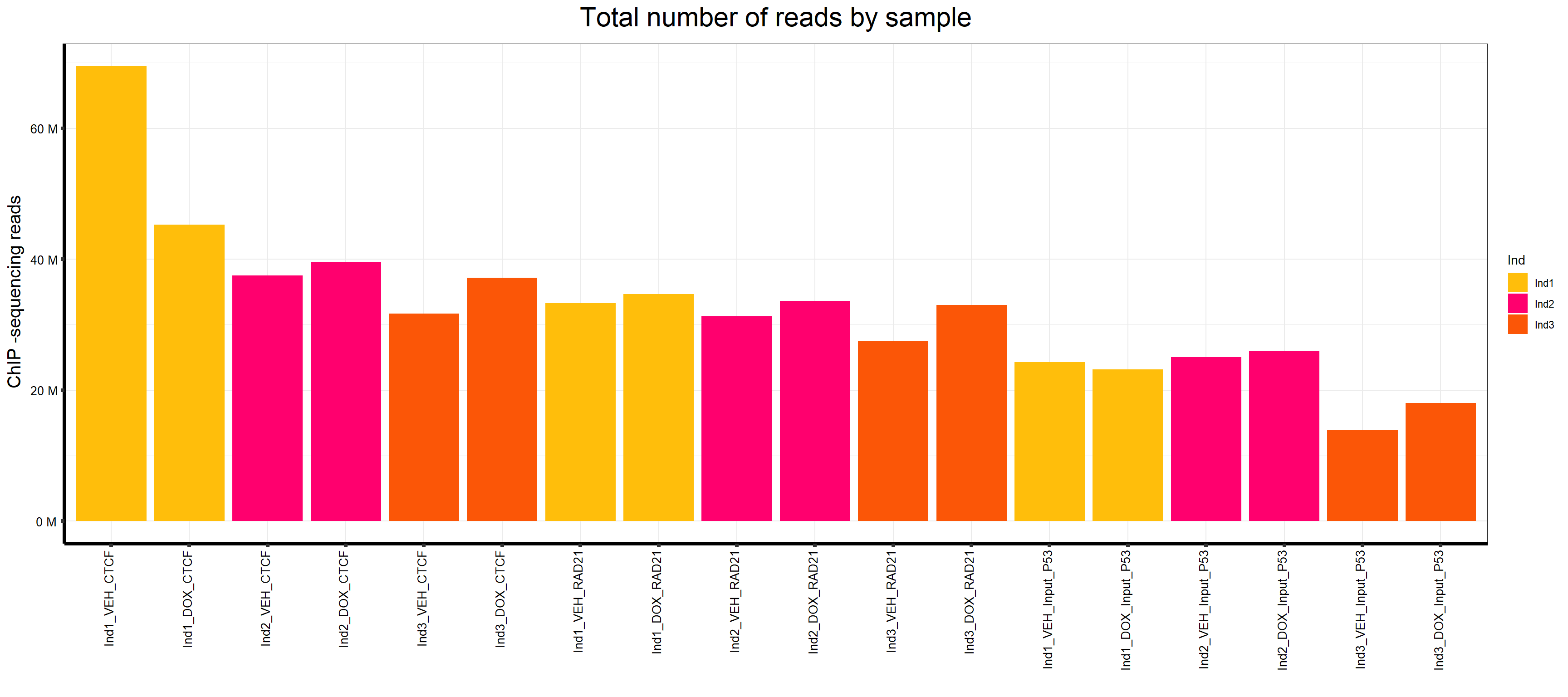
| Version | Author | Date |
|---|---|---|
| 7906757 | sayanpaul01 | 2025-08-15 |
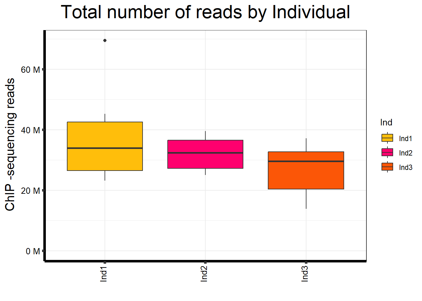
📌 Total Reads by Individuals
map %>%
  ggplot(aes(x = Ind, y = Total.Reads..before.trimming., fill = Ind)) +
  geom_boxplot() +
  scale_fill_manual(values = Ind_palc) +
  scale_y_continuous(labels = label_number(suffix = " M", scale = 1e-6),
                     limits = c(0, NA)) +
  ggtitle(expression("Total number of reads by Individual")) +
  xlab("") +
  ylab(expression("ChIP -sequencing reads")) +
  theme_bw() +
  theme(
    plot.title  = element_text(size = rel(2), hjust = 0.5),
    axis.title  = element_text(size = 15, color = "black"),
    axis.ticks  = element_line(linewidth = 1.5),
    axis.line   = element_line(linewidth = 1.5),
    axis.text.y = element_text(size = 10, color = "black"),
    axis.text.x = element_text(size = 10, color = "black", angle = 90,
                               hjust = 1, vjust = 0.2),
    strip.text.y = element_text(color = "white")
  )
| Version | Author | Date |
|---|---|---|
| 7906757 | sayanpaul01 | 2025-08-15 |
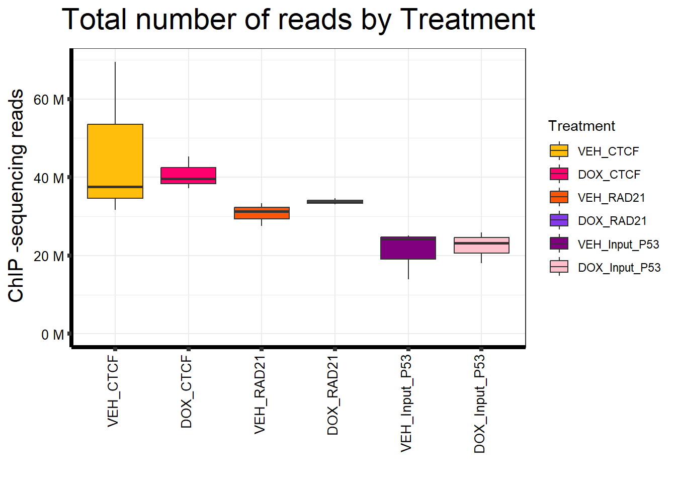
📌 Total Reads by Treatment
map %>%
  ggplot(aes(x = Treatment, y = Total.Reads..before.trimming., fill = Treatment)) +
  geom_boxplot() +
  scale_fill_manual(values = Treat_palc) +
  scale_y_continuous(labels = label_number(suffix = " M", scale = 1e-6),
                     limits = c(0, NA)) +
  ggtitle(expression("Total number of reads by Treatment")) +
  xlab("") +
  ylab(expression("ChIP -sequencing reads")) +
  theme_bw() +
  theme(
    plot.title  = element_text(size = rel(2), hjust = 0.5),
    axis.title  = element_text(size = 15, color = "black"),
    axis.ticks  = element_line(linewidth = 1.5),
    axis.line   = element_line(linewidth = 1.5),
    axis.text.y = element_text(size = 10, color = "black"),
    axis.text.x = element_text(size = 10, color = "black", angle = 90,
                               hjust = 1, vjust = 0.2),
    strip.text.y = element_text(color = "white")
  )
| Version | Author | Date |
|---|---|---|
| 7906757 | sayanpaul01 | 2025-08-15 |
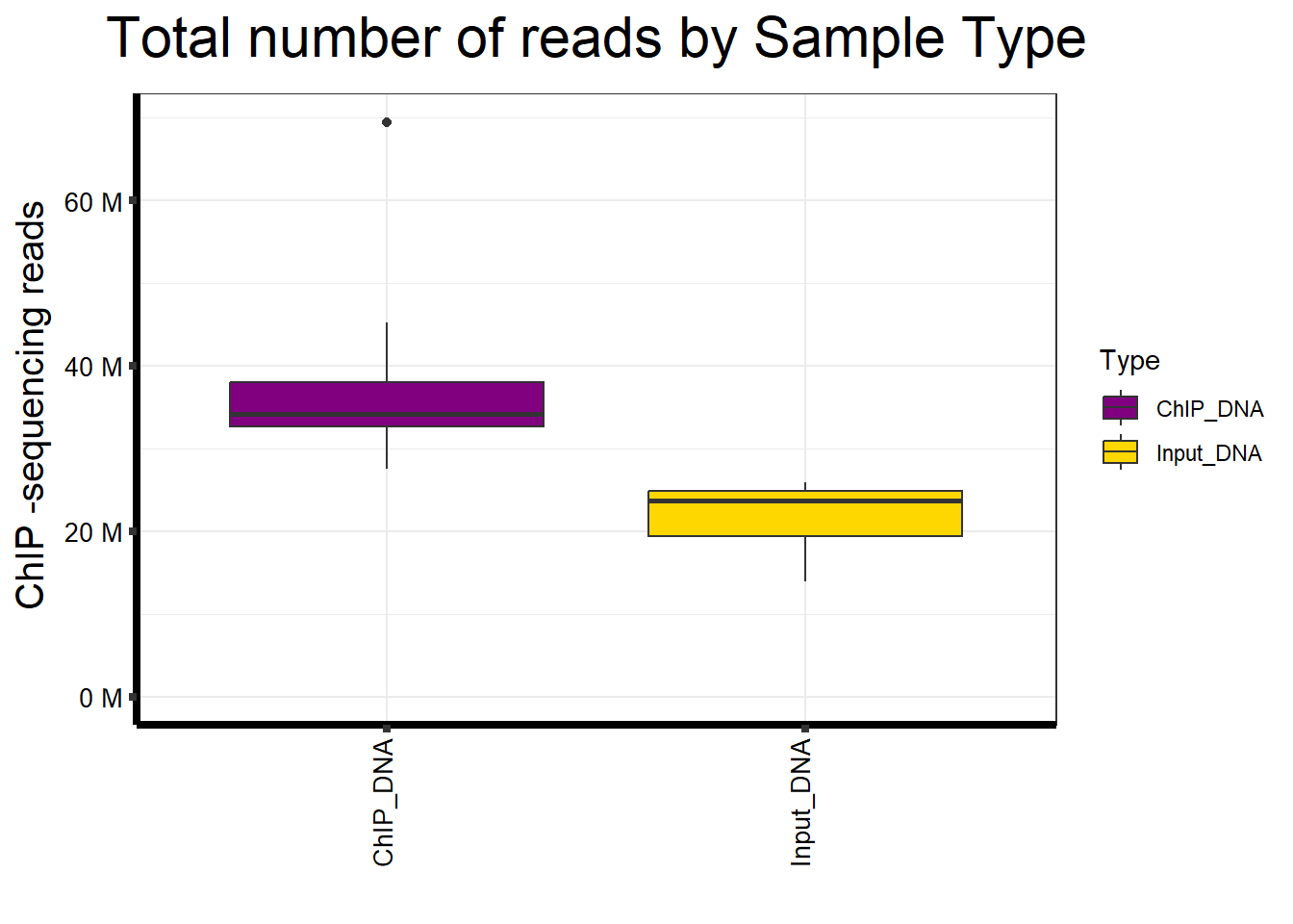
📌 Total Reads by Sample type
map %>%
  ggplot(aes(x = Type, y = Total.Reads..before.trimming., fill = Type)) +
  geom_boxplot() +
  scale_fill_manual(values = Type_palc) +
  scale_y_continuous(labels = label_number(suffix = " M", scale = 1e-6),
                     limits = c(0, NA)) +
  ggtitle(expression("Total number of reads by Sample Type")) +
  xlab("") +
  ylab(expression("ChIP -sequencing reads")) +
  theme_bw() +
  theme(
    plot.title  = element_text(size = rel(2), hjust = 0.5),
    axis.title  = element_text(size = 15, color = "black"),
    axis.ticks  = element_line(linewidth = 1.5),
    axis.line   = element_line(linewidth = 1.5),
    axis.text.y = element_text(size = 10, color = "black"),
    axis.text.x = element_text(size = 10, color = "black", angle = 90,
                               hjust = 1, vjust = 0.2),
    strip.text.y = element_text(color = "white")
  )
| Version | Author | Date |
|---|---|---|
| 7906757 | sayanpaul01 | 2025-08-15 |
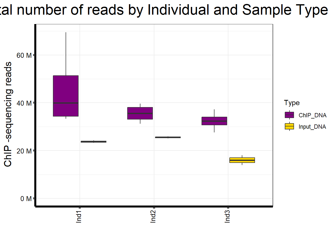
📌 Total Reads by Individuals and Sample type
map %>%
  ggplot(aes(x = Ind, y = Total.Reads..before.trimming., fill = Type)) +
  geom_boxplot() +
  scale_fill_manual(values = Type_palc) +
  scale_y_continuous(labels = label_number(suffix = " M", scale = 1e-6),
                     limits = c(0, NA)) +
  ggtitle(expression("Total number of reads by Individual and Sample Type")) +
  xlab("") +
  ylab(expression("ChIP -sequencing reads")) +
  theme_bw() +
  theme(
    plot.title  = element_text(size = rel(2), hjust = 0.5),
    axis.title  = element_text(size = 15, color = "black"),
    axis.ticks  = element_line(linewidth = 1.5),
    axis.line   = element_line(linewidth = 1.5),
    axis.text.y = element_text(size = 10, color = "black"),
    axis.text.x = element_text(size = 10, color = "black", angle = 90,
                               hjust = 1, vjust = 0.2),
    strip.text.y = element_text(color = "white")
  )
| Version | Author | Date |
|---|---|---|
| 7906757 | sayanpaul01 | 2025-08-15 |
📌 Number of reads before and after trimming
library(dplyr)
library(tidyr)
library(ggplot2)
library(scales)

# Keep sample order as in file
map$Sample.Det <- factor(map$Sample.Det, levels = map$Sample.Det)

# Make sure read counts are numeric (in case CSV parsed as character)
map <- map %>%
  mutate(
    `Total.Reads..before.trimming.` = as.numeric(`Total.Reads..before.trimming.`),
    `Total.reads..after.Trimming.`  = as.numeric(`Total.reads..after.Trimming.`)
  )

# Compute kept fraction for annotation
map <- map %>%
  mutate(kept_frac = `Total.reads..after.Trimming.` / `Total.Reads..before.trimming.`)

# Long format for before vs after
map_long <- map %>%
  pivot_longer(
    cols = c(`Total.Reads..before.trimming.`, `Total.reads..after.Trimming.`),
    names_to = "TrimStage", values_to = "Reads"
  ) %>%
  mutate(
    TrimStage = factor(
      TrimStage,
      levels = c("Total.Reads..before.trimming.", "Total.reads..after.Trimming."),
      labels = c("Before trimming", "After trimming")
    )
  )

# High-contrast (colorblind-safe) colors
stage_colors <- c("Before trimming" = "#1f78b4",  # deep blue
                  "After trimming"  = "#ff7f00")  # bright orange

# Base plot
p <- ggplot(map_long, aes(x = Sample.Det, y = Reads, fill = TrimStage)) +
  geom_col(position = position_dodge(width = 0.8), width = 0.75, color = "black") +
  scale_fill_manual(values = stage_colors) +
  scale_y_continuous(labels = label_number(suffix = " M", scale = 1e-6)) +
  ggtitle(expression("Total number of reads by sample: before vs after trimming")) +
  xlab("") +
  ylab(expression("ChIP-sequencing reads")) +
  theme_bw() +
  theme(
    plot.title  = element_text(size = rel(2), hjust = 0.5),
    axis.title  = element_text(size = 15, color = "black"),
    axis.ticks  = element_line(linewidth = 1.5),
    axis.line   = element_line(linewidth = 1.5),
    axis.text.y = element_text(size = 10, color = "black"),
    axis.text.x = element_text(size = 10, color = "black", angle = 90, hjust = 1, vjust = 0.2),
    legend.title = element_blank()
  )
p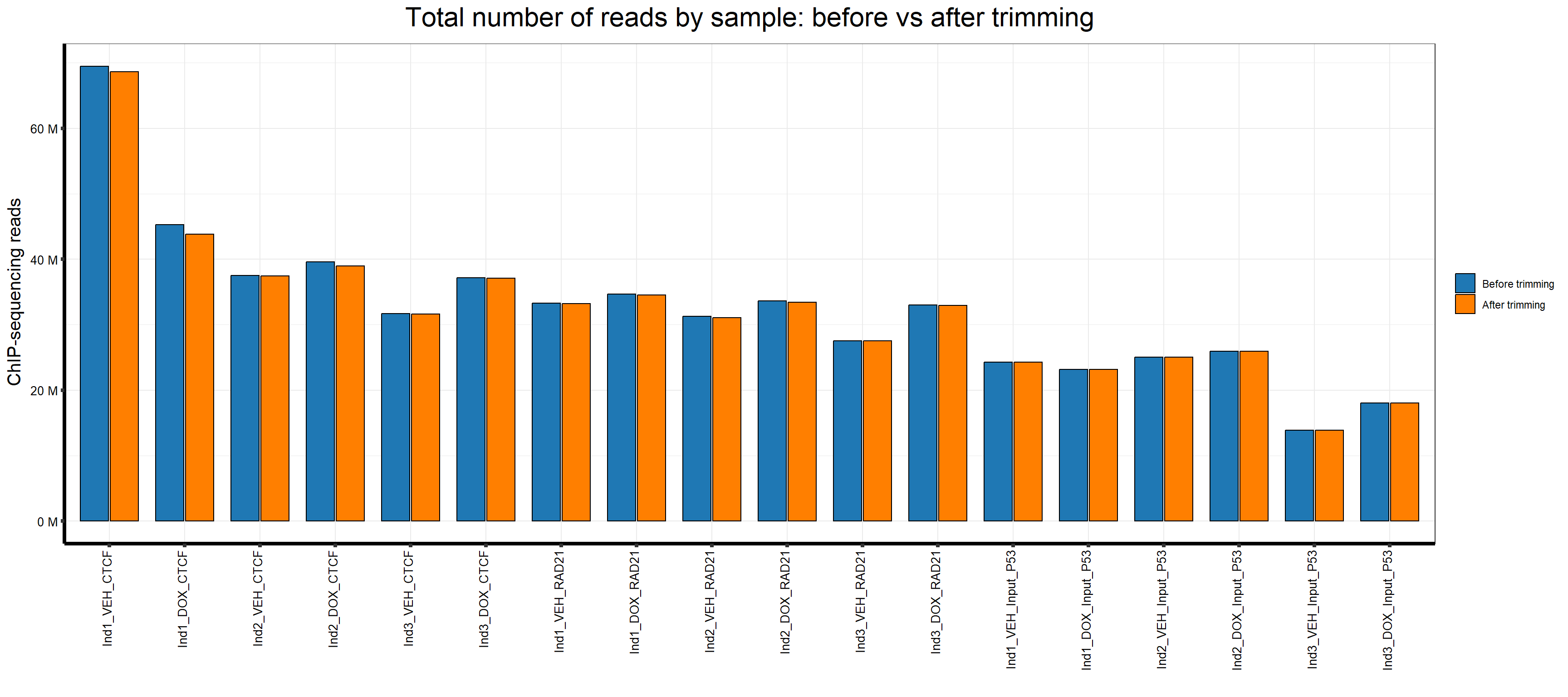
| Version | Author | Date |
|---|---|---|
| 7906757 | sayanpaul01 | 2025-08-15 |
📌 Mean Sequencing Reads Before and After Trimming by Individual, Sample Type, and Antibody
library(dplyr)
library(tidyr)
library(ggplot2)
library(scales)
library(stringr)

# --- Prep -------------------------------------------------------------

# Use your existing data frame name: map (change to df if needed)
df <- map

# Ensure required columns exist / are numeric
df <- df %>%
  mutate(
    `Total.Reads..before.trimming.` = as.numeric(`Total.Reads..before.trimming.`),
    `Total.reads..after.Trimming.`  = as.numeric(`Total.reads..after.Trimming.`)
  )

# Define Tx if your data uses 'Treatment'
if (!"Tx" %in% names(df) && "Treatment" %in% names(df)) {
  df <- df %>% mutate(Tx = Treatment)
}

# Normalize factors you care about
df <- df %>%
  mutate(
    Ab   = ifelse(is.na(Ab) | Ab == "", "Input", as.character(Ab)),
    Type = factor(Type, levels = c("ChIP_DNA", "Input_DNA"))  # adjust if your labels differ
  )

# Helper: label function for Y axis (millions)
reads_lab <- label_number(suffix = " M", scale = 1e-6)

# Kept fraction (After / Before)
df <- df %>%
  mutate(kept_frac = `Total.reads..after.Trimming.` / `Total.Reads..before.trimming.`)

# --- Group, summarise, pivot -----------------------------------------

group_sum <- df %>%
  group_by(Ind, Type, Ab, Tx) %>%
  summarise(
    before_mean = mean(`Total.Reads..before.trimming.`, na.rm = TRUE),
    after_mean  = mean(`Total.reads..after.Trimming.`,  na.rm = TRUE),
    kept_pct    = 100 * mean(kept_frac, na.rm = TRUE),
    .groups     = "drop"
  ) %>%
  pivot_longer(
    cols      = c(before_mean, after_mean),
    names_to  = "stage",
    values_to = "reads"
  ) %>%
  mutate(
    stage = factor(stage, levels = c("before_mean", "after_mean"),
                          labels = c("Before", "After")),
    facet_id = paste0(Ind, "_", Type, "_", Ab)
  )

# Order facets by Ind then Type (cleaner viewing)
facet_levels <- group_sum %>%
  distinct(Ind, Type, Ab, facet_id) %>%
  arrange(Ind, Type, Ab) %>%
  pull(facet_id)

group_sum <- group_sum %>%
  mutate(facet_id = factor(facet_id, levels = facet_levels))

# Optional: prettier strip labels (multi-line)
strip_labeller <- function(ids) {
  parts <- str_split(ids, "_", n = 3, simplify = TRUE)
  paste0("Ind: ", parts[,1], "\nType: ", parts[,2], "\nAb: ", parts[,3])
}

# Colors for Before / After
before_after_colors <- c("Before" = "#1f78b4", "After" = "#ff7f00")

# --- Plot -------------------------------------------------------------

p_group <- ggplot(group_sum, aes(x = Tx, y = reads, fill = stage)) +
  geom_col(position = position_dodge(width = 0.8), width = 0.7, color = "black") +
  scale_fill_manual(values = before_after_colors) +
  facet_wrap(~ facet_id, scales = "free_y",
             labeller = labeller(facet_id = strip_labeller)) +
  scale_y_continuous(labels = reads_lab) +
  labs(
    x = "Treatment",
    y = "Mean reads",
    title = "Mean reads by Individual × Sample Type × Antibody"
  ) +
  theme_bw(base_size = 12) +
  theme(
    legend.title = element_blank(),
    plot.title = element_text(hjust = 0.5, face = "bold"),
    strip.text  = element_text(size = 10)
  )

p_group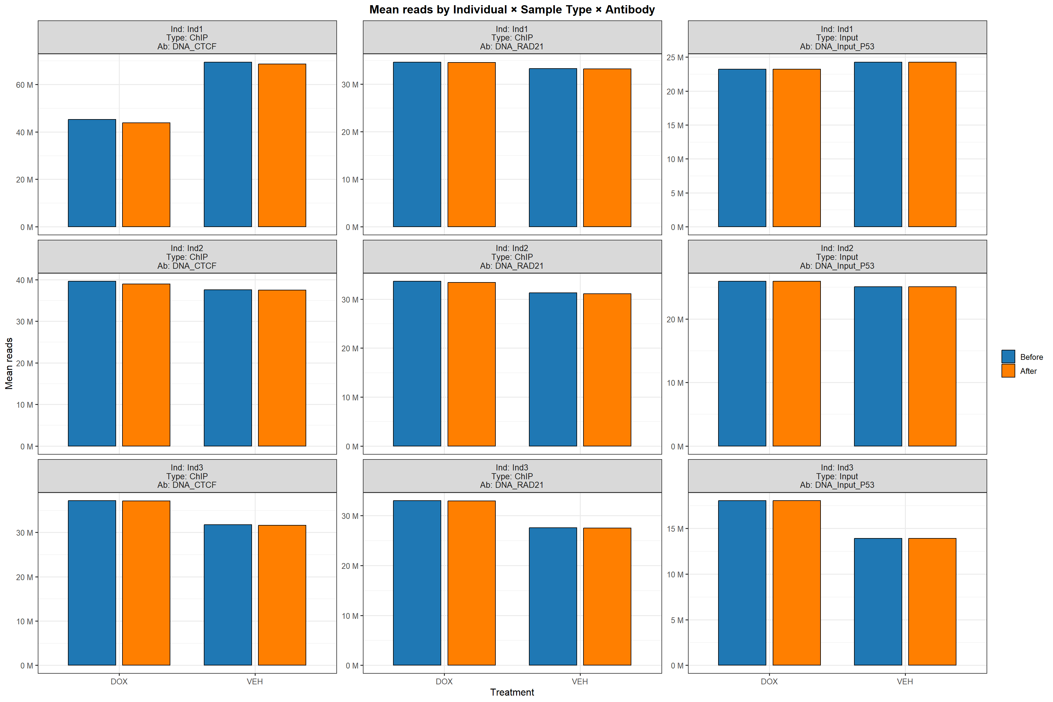
| Version | Author | Date |
|---|---|---|
| 7906757 | sayanpaul01 | 2025-08-15 |
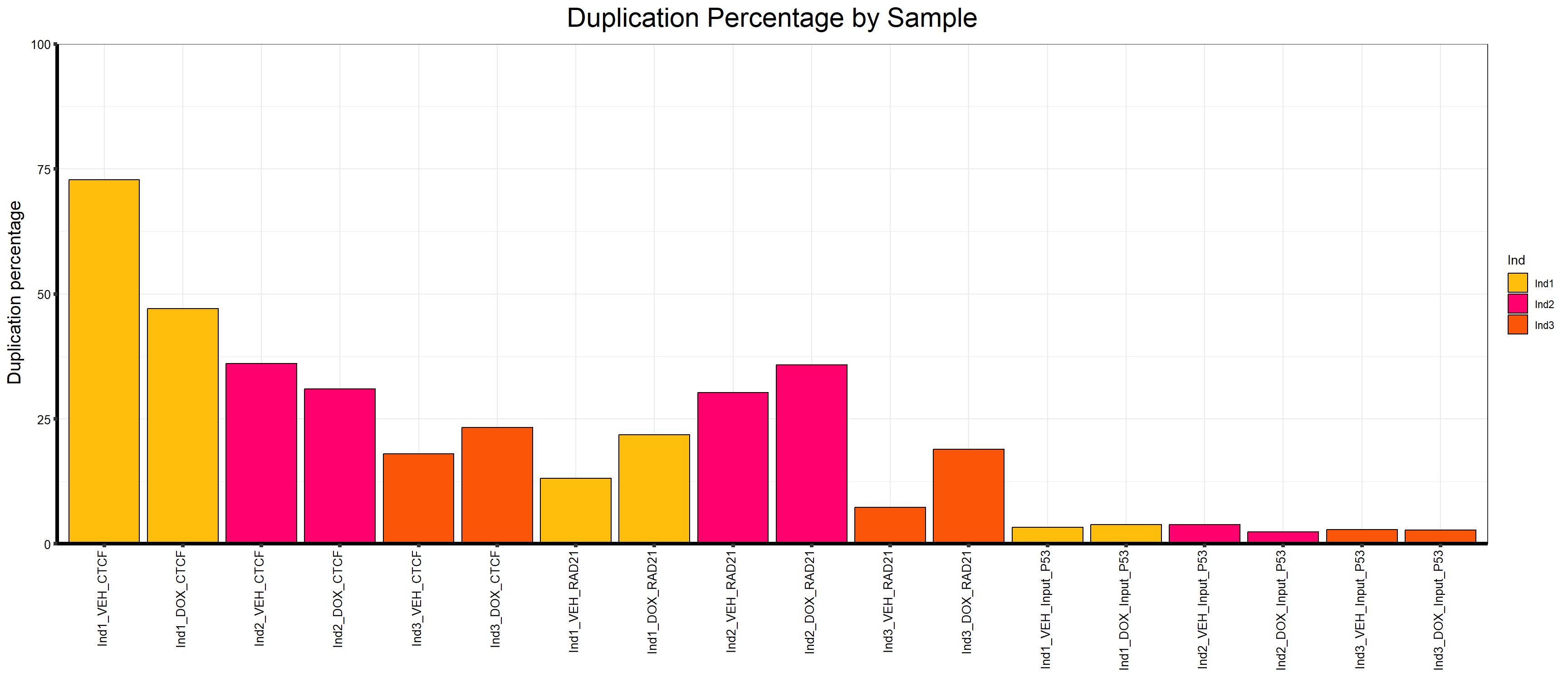
📌 Duplication percentage by Sample
map %>%
  ggplot(aes(x = Sample.Det, y = Duplication.percentage, fill = Ind)) +
  geom_col(color = "black") +
  scale_fill_manual(values = Ind_palc) +
  scale_y_continuous(limits = c(0, 100), expand = c(0, 0)) +
  ggtitle(expression("Duplication Percentage by Sample")) +
  xlab("") +
  ylab(expression("Duplication percentage")) +
  theme_bw() +
  theme(
    plot.title  = element_text(size = rel(2), hjust = 0.5),
    axis.title  = element_text(size = 15, color = "black"),
    axis.ticks  = element_line(linewidth = 1.5),
    axis.line   = element_line(linewidth = 1.5),
    axis.text.y = element_text(size = 10, color = "black"),
    axis.text.x = element_text(size = 10, color = "black", angle = 90,
                               hjust = 1, vjust = 0.2),
    strip.text.y = element_text(color = "white")
  )
| Version | Author | Date |
|---|---|---|
| 7906757 | sayanpaul01 | 2025-08-15 |
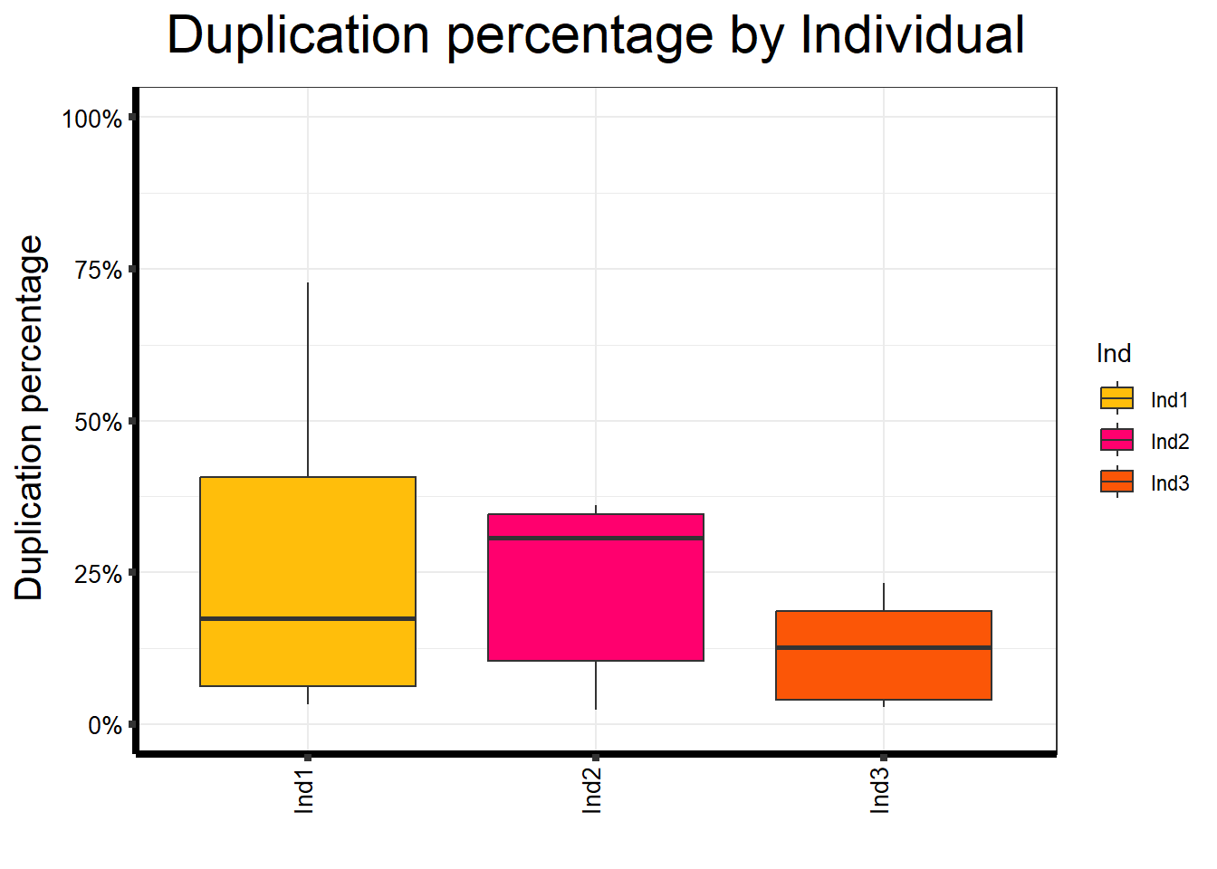
📌 Duplication percentage by Individual
map %>%
  ggplot(aes(x = Ind, y = Duplication.percentage, fill = Ind)) +
  geom_boxplot() +
  scale_fill_manual(values = Ind_palc) +
  scale_y_continuous(limits = c(0, 100), labels = function(x) paste0(x, "%")) +
  ggtitle(expression("Duplication percentage by Individual")) +
  xlab("") +
  ylab(expression("Duplication percentage")) +
  theme_bw() +
  theme(
    plot.title  = element_text(size = rel(2), hjust = 0.5),
    axis.title  = element_text(size = 15, color = "black"),
    axis.ticks  = element_line(linewidth = 1.5),
    axis.line   = element_line(linewidth = 1.5),
    axis.text.y = element_text(size = 10, color = "black"),
    axis.text.x = element_text(size = 10, color = "black", angle = 90,
                               hjust = 1, vjust = 0.2),
    strip.text.y = element_text(color = "white")
  )
| Version | Author | Date |
|---|---|---|
| 7906757 | sayanpaul01 | 2025-08-15 |
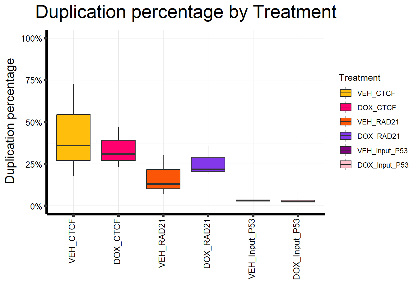
📌 Duplication percentage by Treatment
map %>%
  ggplot(aes(x = Treatment, y = Duplication.percentage, fill = Treatment)) +
  geom_boxplot() +
  scale_fill_manual(values = Treat_palc) +
  scale_y_continuous(limits = c(0, 100), labels = function(x) paste0(x, "%")) +
  ggtitle(expression("Duplication percentage by Treatment")) +
  xlab("") +
  ylab(expression("Duplication percentage")) +
  theme_bw() +
  theme(
    plot.title  = element_text(size = rel(2), hjust = 0.5),
    axis.title  = element_text(size = 15, color = "black"),
    axis.ticks  = element_line(linewidth = 1.5),
    axis.line   = element_line(linewidth = 1.5),
    axis.text.y = element_text(size = 10, color = "black"),
    axis.text.x = element_text(size = 10, color = "black", angle = 90,
                               hjust = 1, vjust = 0.2),
    strip.text.y = element_text(color = "white")
  )
| Version | Author | Date |
|---|---|---|
| 7906757 | sayanpaul01 | 2025-08-15 |
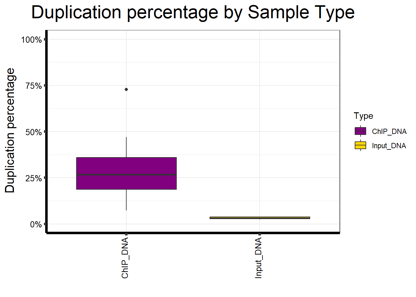
📌 Duplication percentage by Sample type
map %>%
  ggplot(aes(x = Type, y = Duplication.percentage, fill = Type)) +
  geom_boxplot() +
  scale_fill_manual(values = Type_palc) +
  scale_y_continuous(limits = c(0, 100), labels = function(x) paste0(x, "%")) +
  ggtitle(expression("Duplication percentage by Sample Type")) +
  xlab("") +
  ylab(expression("Duplication percentage")) +
  theme_bw() +
  theme(
    plot.title  = element_text(size = rel(2), hjust = 0.5),
    axis.title  = element_text(size = 15, color = "black"),
    axis.ticks  = element_line(linewidth = 1.5),
    axis.line   = element_line(linewidth = 1.5),
    axis.text.y = element_text(size = 10, color = "black"),
    axis.text.x = element_text(size = 10, color = "black", angle = 90,
                               hjust = 1, vjust = 0.2),
    strip.text.y = element_text(color = "white")
  )
| Version | Author | Date |
|---|---|---|
| 7906757 | sayanpaul01 | 2025-08-15 |
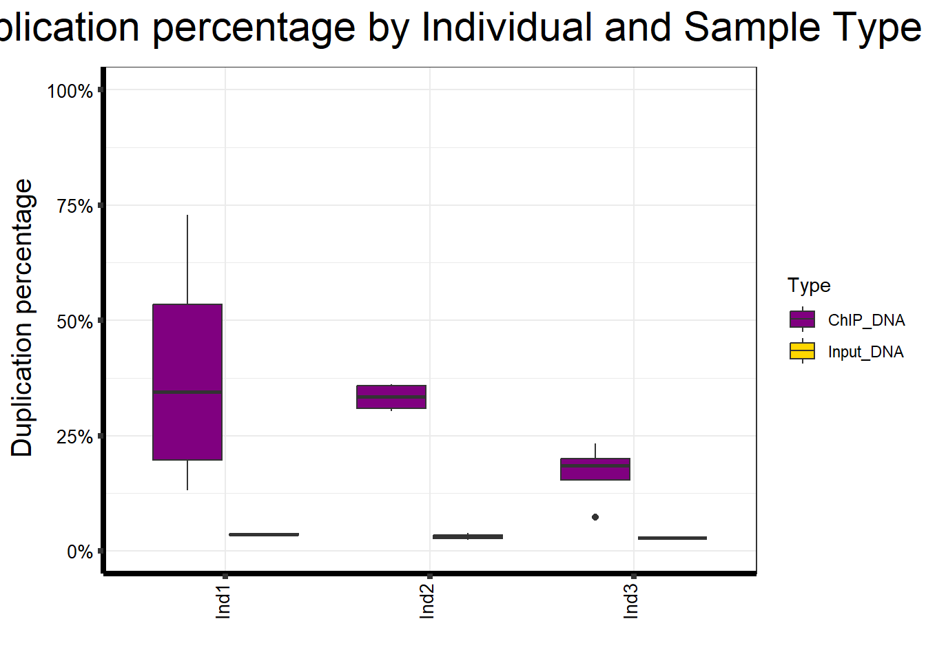
📌 Duplication percentage by Individual and Sample type
map %>%
  ggplot(aes(x = Ind, y = Duplication.percentage, fill = Type)) +
  geom_boxplot() +
  scale_fill_manual(values = Type_palc) +
  scale_y_continuous(limits = c(0, 100), labels = function(x) paste0(x, "%")) +
  ggtitle(expression("Duplication percentage by Individual and Sample Type")) +
  xlab("") +
  ylab(expression("Duplication percentage")) +
  theme_bw() +
  theme(
    plot.title  = element_text(size = rel(2), hjust = 0.5),
    axis.title  = element_text(size = 15, color = "black"),
    axis.ticks  = element_line(linewidth = 1.5),
    axis.line   = element_line(linewidth = 1.5),
    axis.text.y = element_text(size = 10, color = "black"),
    axis.text.x = element_text(size = 10, color = "black", angle = 90,
                               hjust = 1, vjust = 0.2),
    strip.text.y = element_text(color = "white")
  )
| Version | Author | Date |
|---|---|---|
| 7906757 | sayanpaul01 | 2025-08-15 |
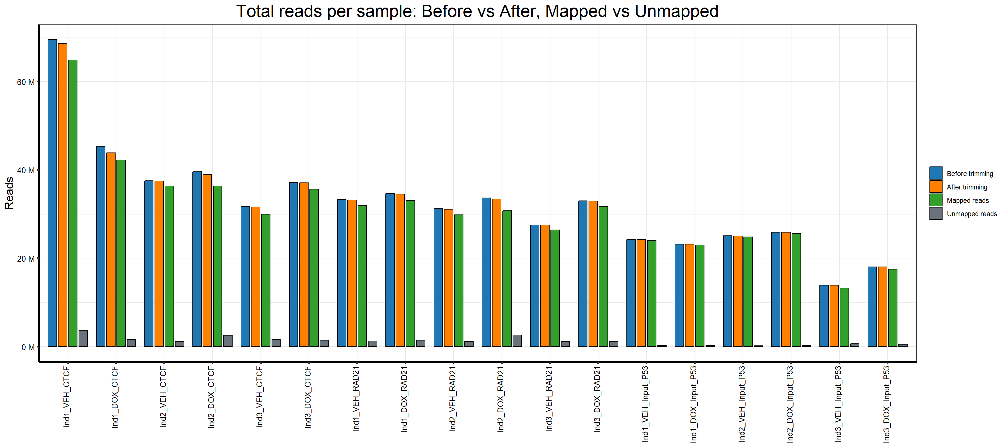
📌 Mapping Summary
library(dplyr)
library(tidyr)
library(ggplot2)
library(scales)

# If not already done, read with check.names=TRUE so we have dot-style names
# map <- read.csv("data/ChIP Seq Summary stat TOP2B P53.csv", check.names = TRUE)

# Keep sample order as in the file
map$Sample.Det <- factor(map$Sample.Det, levels = map$Sample.Det)

# Ensure numeric (CSV can import as character)
map <- map %>%
  mutate(
    Total.Reads..before.trimming. = as.numeric(Total.Reads..before.trimming.),
    Total.reads..after.Trimming.  = as.numeric(Total.reads..after.Trimming.),
    Mapped.Reads                  = as.numeric(Mapped.Reads),
    Unmapped.reads                = as.numeric(Unmapped.reads)
  )

# Long format for the 4 metrics
metric_order <- c("Total.Reads..before.trimming.",
                  "Total.reads..after.Trimming.",
                  "Mapped.Reads",
                  "Unmapped.reads")

map_long4 <- map %>%
  dplyr::select(Sample.Det, all_of(metric_order)) %>%
  pivot_longer(cols = all_of(metric_order), names_to = "Metric", values_to = "Reads") %>%
  mutate(
    Metric = factor(
      Metric,
      levels = metric_order,
      labels = c("Before trimming", "After trimming", "Mapped reads", "Unmapped reads")
    )
  )


# Colors (colorblind-friendly)
metric_cols <- c(
  "Before trimming" = "#1f78b4",  # blue
  "After trimming"  = "#ff7f00",  # orange
  "Mapped reads"    = "#33a02c",  # green
  "Unmapped reads"  = "#6a737b"   # gray
)

# Plot: grouped bars per sample
ggplot(map_long4, aes(x = Sample.Det, y = Reads, fill = Metric)) +
  geom_col(position = position_dodge(width = 0.85), width = 0.72, color = "black") +
  scale_fill_manual(values = metric_cols) +
  scale_y_continuous(labels = label_number(suffix = " M", scale = 1e-6)) +
  labs(
    title = "Total reads per sample: Before vs After, Mapped vs Unmapped",
    x = NULL,
    y = "Reads"
  ) +
  theme_bw() +
  theme(
    plot.title  = element_text(size = rel(2), hjust = 0.5),
    axis.title  = element_text(size = 15, color = "black"),
    axis.ticks  = element_line(linewidth = 1.2),
    axis.line   = element_line(linewidth = 1.2),
    axis.text.y = element_text(size = 10, color = "black"),
    axis.text.x = element_text(size = 10, color = "black", angle = 90, hjust = 1, vjust = 0.2),
    legend.title = element_blank()
  )
| Version | Author | Date |
|---|---|---|
| 90183c3 | sayanpaul01 | 2025-08-17 |
📌 Total, mapped and unmapped reads by individual
library(dplyr)
library(tidyr)
library(ggplot2)
library(scales)

# Keep original dot-style names (assumes you read with check.names=TRUE)
# map <- read.csv("data/ChIP Seq Summary stat TOP2B P53.csv", check.names = TRUE)

# Make sure numeric
map <- map %>%
  mutate(
    Total.Reads..before.trimming. = as.numeric(Total.Reads..before.trimming.),
    Mapped.Reads                 = as.numeric(Mapped.Reads),
    Unmapped.reads               = as.numeric(Unmapped.reads)
  )

comp_cols <- c(
  "Total reads" = "#1f78b4",  # blue
  "Mapped reads"    = "#33a02c",  # green
  "Unmapped reads"  = "#6a737b"   # gray
)


# Long format for the 3 metrics
metric_order  <- c("Total.Reads..before.trimming.", "Mapped.Reads", "Unmapped.reads")
metric_labels <- c("Total reads", "Mapped reads", "Unmapped reads")

map_long3 <- map %>%
  pivot_longer(
    cols = all_of(metric_order),
    names_to = "Metric",
    values_to = "Reads"
  ) %>%
  mutate(
    Metric = factor(Metric, levels = metric_order, labels = metric_labels)
  )


ggplot(map_long3, aes(x = Ind, y = Reads, fill = Metric)) +
  geom_boxplot(position = position_dodge(width = 0.75)) +
  scale_fill_manual(values = comp_cols) +
  scale_y_continuous(labels = label_number(suffix = " M", scale = 1e-6)) +
  labs(title = "Reads by Individual: Total, mapped and Unmapped",
       x = NULL, y = "Reads") +
  theme_bw() +
  theme(plot.title = element_text(size = rel(1.8), hjust = 0.5),
        legend.title = element_blank(),
        axis.text.x = element_text(angle = 90, hjust = 1, vjust = 0.2))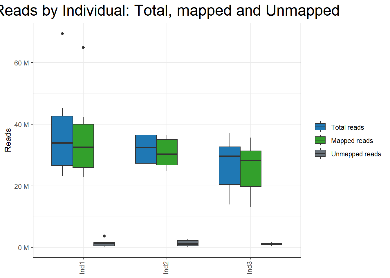
| Version | Author | Date |
|---|---|---|
| 90183c3 | sayanpaul01 | 2025-08-17 |
📌 Total, mapped and unmapped reads by treatment
ggplot(map_long3, aes(x = Treatment, y = Reads, fill = Metric)) +
  geom_boxplot(position = position_dodge(width = 0.75)) +
  scale_fill_manual(values = comp_cols) +
  scale_y_continuous(labels = label_number(suffix = " M", scale = 1e-6)) +
  labs(title = "Reads by Treatment: Total, mapped and Unmapped",
       x = NULL, y = "Reads") +
  theme_bw() +
  theme(plot.title = element_text(size = rel(1.8), hjust = 0.5),
        legend.title = element_blank(),
        axis.text.x = element_text(angle = 90, hjust = 1, vjust = 0.2))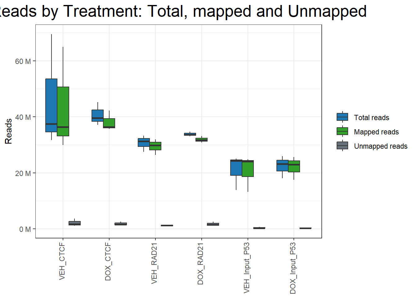
| Version | Author | Date |
|---|---|---|
| 90183c3 | sayanpaul01 | 2025-08-17 |
📌 Total, mapped and unmapped reads by Sample type
ggplot(map_long3, aes(x = Type, y = Reads, fill = Metric)) +
  geom_boxplot(position = position_dodge(width = 0.75)) +
  scale_fill_manual(values = comp_cols) +
  scale_y_continuous(labels = label_number(suffix = " M", scale = 1e-6)) +
  labs(title = "Reads by Sample Type: Total, mapped and Unmapped",
       x = NULL, y = "Reads") +
  theme_bw() +
  theme(plot.title = element_text(size = rel(1.8), hjust = 0.5),
        legend.title = element_blank(),
        axis.text.x = element_text(angle = 90, hjust = 1, vjust = 0.2))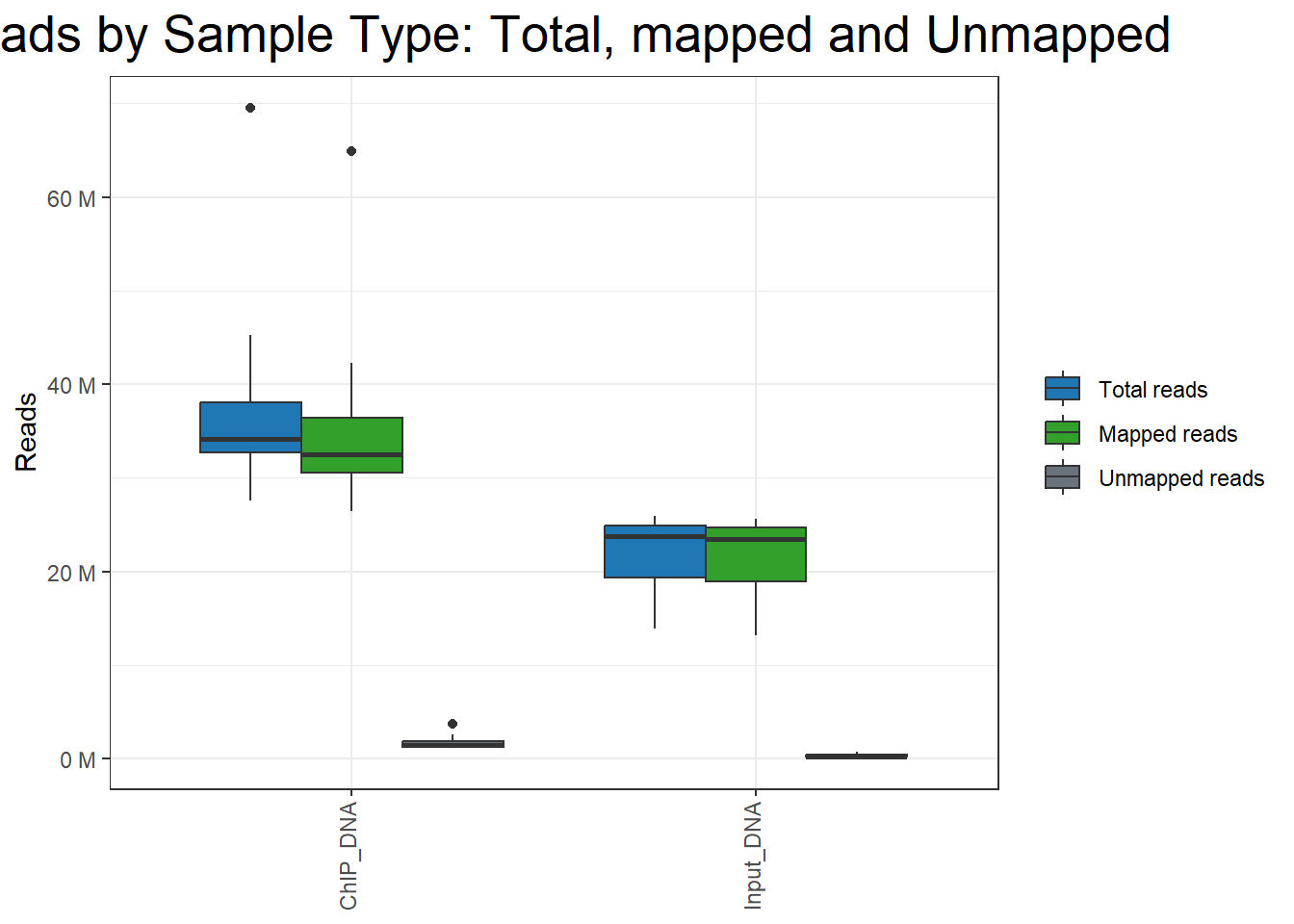
| Version | Author | Date |
|---|---|---|
| 90183c3 | sayanpaul01 | 2025-08-17 |
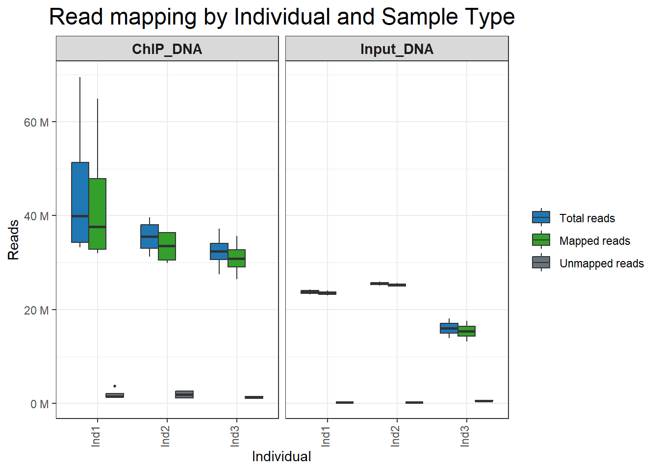
📌 Total, mapped and unmapped reads by individual and sample type
library(dplyr)
library(tidyr)
library(ggplot2)
library(scales)

# Make sure numeric
map <- map %>%
  mutate(
    Total.Reads..before.trimming. = as.numeric(Total.Reads..before.trimming.),
    Mapped.Reads                  = as.numeric(Mapped.Reads),
    Unmapped.reads                = as.numeric(Unmapped.reads)
  )

# Colors for boxplot fill
comp_cols <- c(
  "Total reads" = "#1f78b4",  # blue
  "Mapped reads"    = "#33a02c",  # green
  "Unmapped reads"  = "#6a737b"   # gray
)


# Reshape into long format
map_long <- map %>%
  dplyr::select(Ind, Type,
                Total.Reads..before.trimming., Mapped.Reads, Unmapped.reads) %>%
  tidyr::pivot_longer(
    cols = c(Total.Reads..before.trimming., Mapped.Reads, Unmapped.reads),
    names_to = "Metric", values_to = "Reads"
  ) %>%
  dplyr::mutate(
    Metric = factor(Metric,
      levels = c("Total.Reads..before.trimming.", "Mapped.Reads", "Unmapped.reads"),
      labels = c("Total reads", "Mapped reads", "Unmapped reads"))
  )

# ---- Plot ----
ggplot(map_long, aes(x = Ind, y = Reads, fill = Metric)) +
  geom_boxplot(outlier.size = 0.8, position = position_dodge(width = 0.75)) +
  scale_fill_manual(values = comp_cols) +
  scale_y_continuous(labels = label_number(suffix = " M", scale = 1e-6)) +
  facet_wrap(~ Type) +
  labs(
    title = "Read mapping by Individual and Sample Type",
    x = "Individual", y = "Reads"
  ) +
  theme_bw() +
  theme(
    plot.title   = element_text(size = rel(1.6), hjust = 0.5),
    legend.title = element_blank(),
    strip.text   = element_text(size = 11, face = "bold"),
    axis.text.x  = element_text(angle = 90, hjust = 1, vjust = 0.2)
  )
| Version | Author | Date |
|---|---|---|
| 90183c3 | sayanpaul01 | 2025-08-17 |
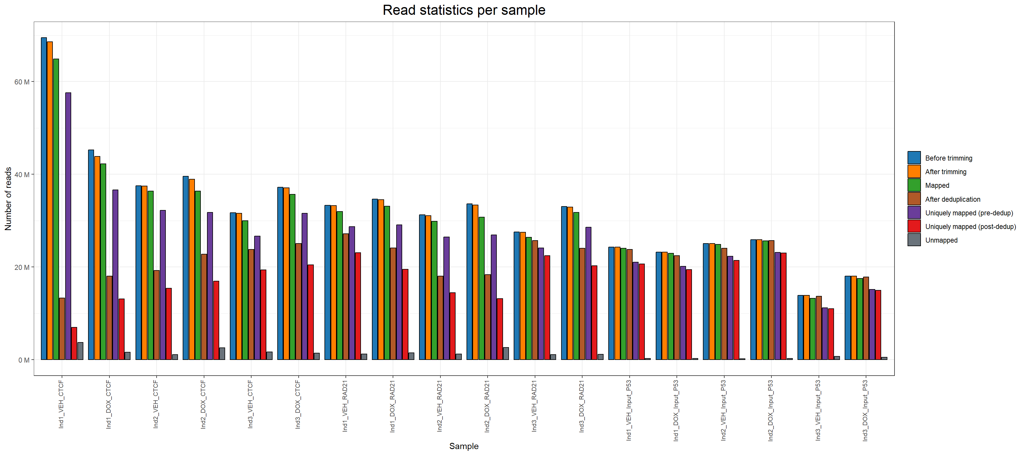
📌 Total, Mapped, Unmapped, and Deduplicated and uniquely mapped Reads per Sample
library(dplyr)
library(tidyr)
library(ggplot2)
library(scales)

# ---- Load data (already read into "map") ----
# If needed, uncomment the following line to read fresh:
# map <- read.csv("data/ChIP Seq Summary stat TOP2B P53.csv", check.names = TRUE)

# Convert to tibble for tidyverse
map <- tibble::as_tibble(map)

# Keep sample order as in the file
map$Sample.Det <- factor(map$Sample.Det, levels = map$Sample.Det)

# Ensure numeric for all metrics
map <- map %>%
  mutate(
    Total.Reads..before.trimming.              = as.numeric(Total.Reads..before.trimming.),
    Total.reads..after.Trimming.               = as.numeric(Total.reads..after.Trimming.),
    Mapped.Reads                               = as.numeric(Mapped.Reads),
    Reads.after.deduplication                  = as.numeric(Reads.after.deduplication),
    Uniquely.mapped.reads.before.deduplication = as.numeric(Uniquely.mapped.reads.before.deduplication),
    Uniquely.mapped.reads.after.deduplication  = as.numeric(Uniquely.mapped.reads.after.deduplication),
    Unmapped.reads                             = as.numeric(Unmapped.reads)
  )

# ---- Define order, labels, and colors ----
metric_order <- c(
  "Total.Reads..before.trimming.",
  "Total.reads..after.Trimming.",
  "Mapped.Reads",
  "Reads.after.deduplication",
  "Uniquely.mapped.reads.before.deduplication",
  "Uniquely.mapped.reads.after.deduplication",
  "Unmapped.reads"
)

metric_labels <- c(
  "Total.Reads..before.trimming."              = "Before trimming",
  "Total.reads..after.Trimming."               = "After trimming",
  "Mapped.Reads"                               = "Mapped",
  "Reads.after.deduplication"                  = "After deduplication",
  "Uniquely.mapped.reads.before.deduplication" = "Uniquely mapped (pre-dedup)",
  "Uniquely.mapped.reads.after.deduplication"  = "Uniquely mapped (post-dedup)",
  "Unmapped.reads"                             = "Unmapped"
)

metric_colors <- c(
  "Before trimming"              = "#1f78b4",  # blue
  "After trimming"               = "#ff7f00",  # orange
  "Mapped"                       = "#33a02c",  # green
  "After deduplication"          = "#b15928",  # brown
  "Uniquely mapped (pre-dedup)"  = "#6a3d9a",  # purple
  "Uniquely mapped (post-dedup)" = "#e31a1c",  # red
  "Unmapped"                     = "#6a737b"   # gray
)

# ---- Reshape to long format ----
map_long <- map %>%
  dplyr::select(Sample.Det, dplyr::all_of(metric_order)) %>%
  tidyr::pivot_longer(
    cols = dplyr::all_of(metric_order),
    names_to = "Metric", values_to = "Reads"
  ) %>%
  dplyr::mutate(
    Metric = factor(Metric, levels = metric_order, labels = metric_labels)
  )


# ---- Plot ----
ggplot(map_long, aes(x = Sample.Det, y = Reads, fill = Metric)) +
  geom_col(position = position_dodge(width = 0.9), width = 0.8, color = "black") +
  scale_fill_manual(values = metric_colors) +
  scale_y_continuous(labels = label_number(suffix = " M", scale = 1e-6)) +
  labs(
    title = "Read statistics per sample",
    x = "Sample",
    y = "Number of reads"
  ) +
  theme_bw() +
  theme(
    plot.title   = element_text(size = rel(1.6), hjust = 0.5),
    axis.text.x  = element_text(size = 8, angle = 90, hjust = 1, vjust = 0.2),
    legend.title = element_blank()
  )
| Version | Author | Date |
|---|---|---|
| ab9a136 | sayanpaul01 | 2025-08-18 |
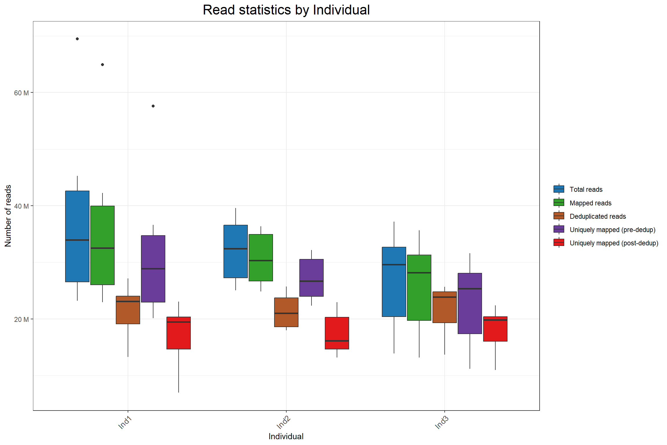
📌 Total, Mapped, Unmapped, and Deduplicated and uniquely mapped Reads per Individual
library(dplyr)
library(tidyr)
library(ggplot2)
library(scales)

# ---- Make sure numeric ----
map <- map %>%
  mutate(
    Total.Reads..before.trimming.              = as.numeric(Total.Reads..before.trimming.),
    Mapped.Reads                               = as.numeric(Mapped.Reads),
    Reads.after.deduplication                  = as.numeric(Reads.after.deduplication),
    Uniquely.mapped.reads.before.deduplication = as.numeric(Uniquely.mapped.reads.before.deduplication),
    Uniquely.mapped.reads.after.deduplication  = as.numeric(Uniquely.mapped.reads.after.deduplication)
  )

# ---- Define order, labels, and colors ----
metric_order <- c(
  "Total.Reads..before.trimming.",
  "Mapped.Reads",
  "Reads.after.deduplication",
  "Uniquely.mapped.reads.before.deduplication",
  "Uniquely.mapped.reads.after.deduplication"
)

metric_labels <- c(
  "Total.Reads..before.trimming."              = "Total reads",
  "Mapped.Reads"                               = "Mapped reads",
  "Reads.after.deduplication"                  = "Deduplicated reads",
  "Uniquely.mapped.reads.before.deduplication" = "Uniquely mapped (pre-dedup)",
  "Uniquely.mapped.reads.after.deduplication"  = "Uniquely mapped (post-dedup)"
)

metric_colors <- c(
  "Total reads"                  = "#1f78b4",  # blue
  "Mapped reads"                 = "#33a02c",  # green
  "Deduplicated reads"           = "#b15928",  # brown
  "Uniquely mapped (pre-dedup)"  = "#6a3d9a",  # purple
  "Uniquely mapped (post-dedup)" = "#e31a1c"   # red
)

# ---- Reshape to long format ----
map_long <- map %>%
  dplyr::select(Ind, dplyr::all_of(metric_order)) %>%
  tidyr::pivot_longer(cols = dplyr::all_of(metric_order),
               names_to = "Metric", values_to = "Reads") %>%
  dplyr::mutate(
    Metric = factor(Metric, levels = metric_order, labels = metric_labels)
  )

# ---- Plot ----
ggplot(map_long, aes(x = Ind, y = Reads, fill = Metric)) +
  geom_boxplot(position = position_dodge(width = 0.8)) +
  scale_fill_manual(values = metric_colors) +
  scale_y_continuous(labels = label_number(suffix = " M", scale = 1e-6)) +
  labs(
    title = "Read statistics by Individual",
    x = "Individual",
    y = "Number of reads"
  ) +
  theme_bw() +
  theme(
    plot.title   = element_text(size = rel(1.6), hjust = 0.5),
    legend.title = element_blank(),
    axis.text.x  = element_text(size = 10, angle = 45, hjust = 1)
  )
| Version | Author | Date |
|---|---|---|
| ab9a136 | sayanpaul01 | 2025-08-18 |
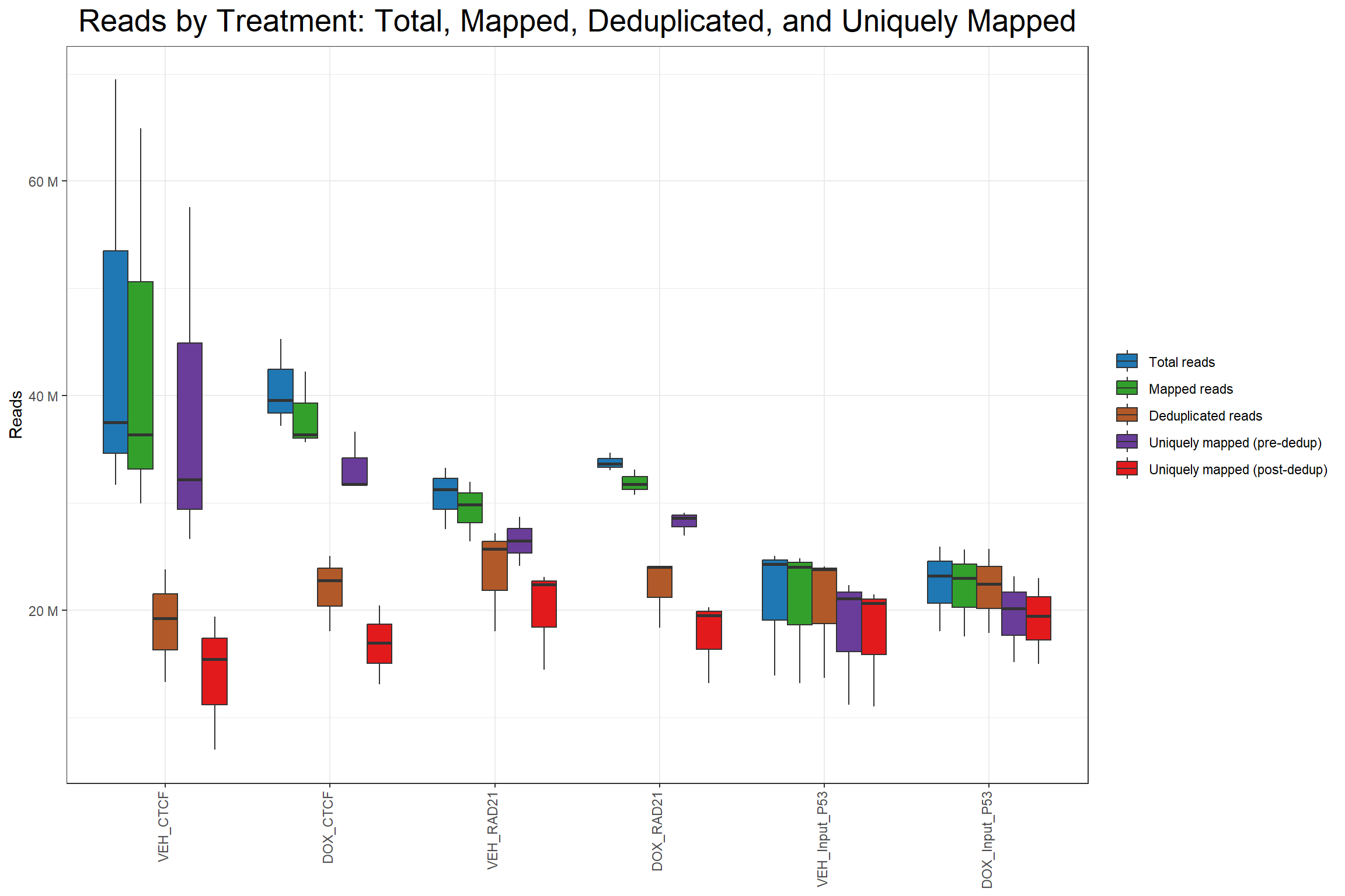
📌 Total, Mapped, Unmapped, and Deduplicated and uniquely mapped Reads per treatment
# ---- Long format ----
map_long_tx <- map %>%
  dplyr::select(Treatment, dplyr::all_of(metric_order)) %>%
  tidyr::pivot_longer(
    cols = dplyr::all_of(metric_order),
    names_to = "Metric", values_to = "Reads"
  ) %>%
  dplyr::mutate(
    Metric = factor(Metric, levels = metric_order, labels = metric_labels)
  )

# ---- Plot ----
ggplot(map_long_tx, aes(x = Treatment, y = Reads, fill = Metric)) +
  geom_boxplot(position = position_dodge(width = 0.75)) +
  scale_fill_manual(values = metric_colors) +
  scale_y_continuous(labels = label_number(suffix = " M", scale = 1e-6)) +
  labs(
    title = "Reads by Treatment: Total, Mapped, Deduplicated, and Uniquely Mapped",
    x = NULL, y = "Reads"
  ) +
  theme_bw() +
  theme(
    plot.title   = element_text(size = rel(1.8), hjust = 0.5),
    legend.title = element_blank(),
    axis.text.x  = element_text(angle = 90, hjust = 1, vjust = 0.2)
  )
| Version | Author | Date |
|---|---|---|
| ab9a136 | sayanpaul01 | 2025-08-18 |
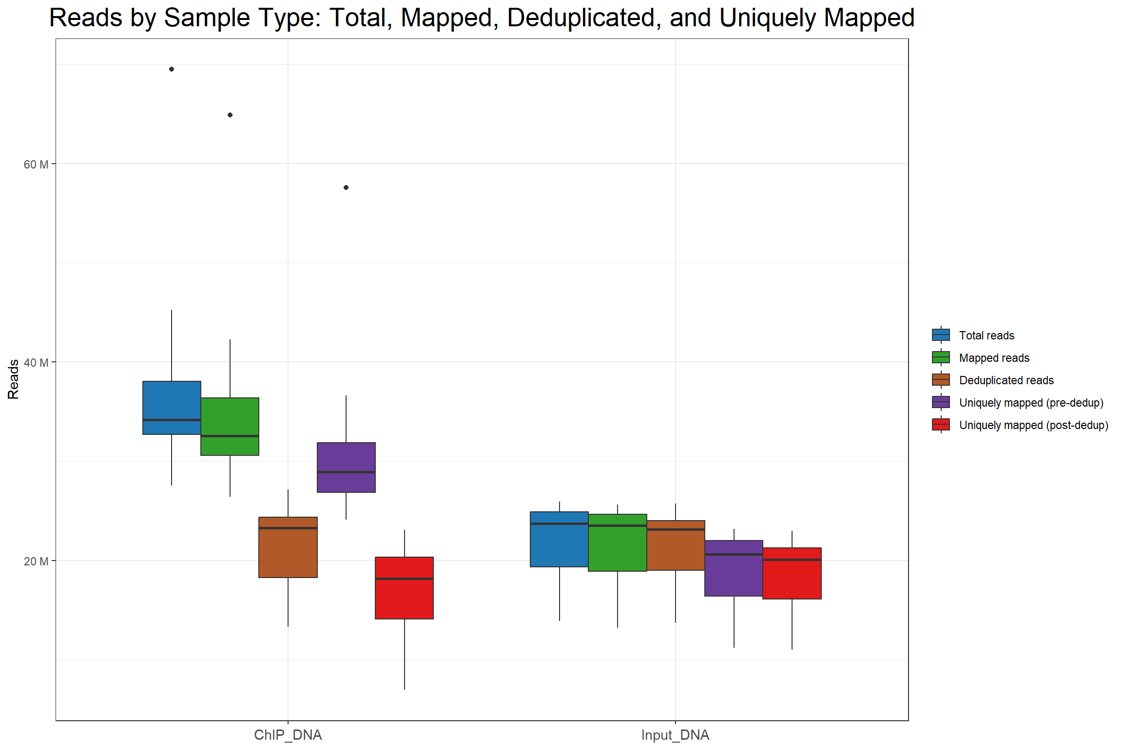
📌 Total, Mapped, Unmapped, and Deduplicated and uniquely mapped Reads per sample type
# ---- Long format by Sample Type ----
map_long_type <- map %>%
  dplyr::select(Type, dplyr::all_of(metric_order)) %>%
  tidyr::pivot_longer(
    cols = dplyr::all_of(metric_order),
    names_to = "Metric", values_to = "Reads"
  ) %>%
  dplyr::mutate(
    Metric = factor(Metric, levels = metric_order, labels = metric_labels)
  )

# ---- Plot ----
ggplot(map_long_type, aes(x = Type, y = Reads, fill = Metric)) +
  geom_boxplot(position = position_dodge(width = 0.75)) +
  scale_fill_manual(values = metric_colors) +
  scale_y_continuous(labels = label_number(suffix = " M", scale = 1e-6)) +
  labs(
    title = "Reads by Sample Type: Total, Mapped, Deduplicated, and Uniquely Mapped",
    x = NULL, y = "Reads"
  ) +
  theme_bw() +
  theme(
    plot.title   = element_text(size = rel(1.8), hjust = 0.5),
    legend.title = element_blank(),
    axis.text.x  = element_text(angle = 0, hjust = 0.5, vjust = 0.5, size = 11)
  )
| Version | Author | Date |
|---|---|---|
| ab9a136 | sayanpaul01 | 2025-08-18 |
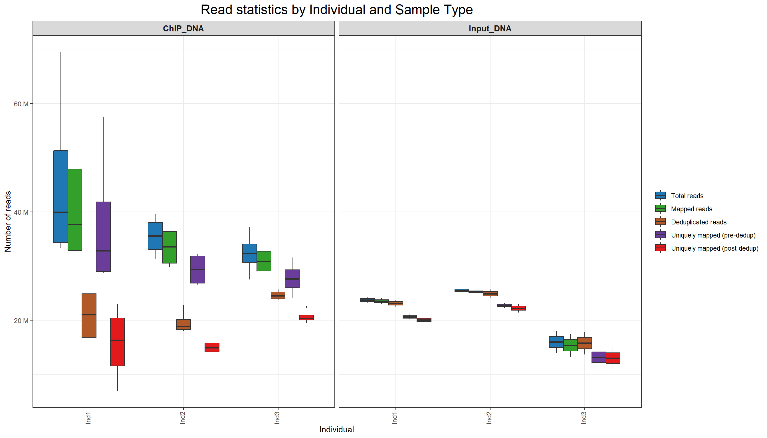
📌 Total, Mapped, Unmapped, and Deduplicated and uniquely mapped Reads per sample type and individuals
library(dplyr)
library(tidyr)
library(ggplot2)
library(scales)

# Make sure numeric
map <- map %>%
  mutate(
    Total.Reads..before.trimming.              = as.numeric(Total.Reads..before.trimming.),
    Mapped.Reads                               = as.numeric(Mapped.Reads),
    Reads.after.deduplication                  = as.numeric(Reads.after.deduplication),
    Uniquely.mapped.reads.before.deduplication = as.numeric(Uniquely.mapped.reads.before.deduplication),
    Uniquely.mapped.reads.after.deduplication  = as.numeric(Uniquely.mapped.reads.after.deduplication)
  )

# Colors for boxplot fill (5 metrics)
comp_cols <- c(
  "Total reads"                  = "#1f78b4",  # blue
  "Mapped reads"                 = "#33a02c",  # green
  "Deduplicated reads"           = "#b15928",  # brown
  "Uniquely mapped (pre-dedup)"  = "#6a3d9a",  # purple
  "Uniquely mapped (post-dedup)" = "#e31a1c"   # red
)

# Reshape into long format
map_long <- map %>%
  dplyr::select(
    Ind, Type,
    Total.Reads..before.trimming., Mapped.Reads,
    Reads.after.deduplication,
    Uniquely.mapped.reads.before.deduplication,
    Uniquely.mapped.reads.after.deduplication
  ) %>%
  tidyr::pivot_longer(
    cols = c(
      Total.Reads..before.trimming., Mapped.Reads,
      Reads.after.deduplication,
      Uniquely.mapped.reads.before.deduplication,
      Uniquely.mapped.reads.after.deduplication
    ),
    names_to = "Metric", values_to = "Reads"
  ) %>%
  dplyr::mutate(
    Metric = factor(
      Metric,
      levels = c(
        "Total.Reads..before.trimming.", "Mapped.Reads",
        "Reads.after.deduplication",
        "Uniquely.mapped.reads.before.deduplication",
        "Uniquely.mapped.reads.after.deduplication"
      ),
      labels = c(
        "Total reads", "Mapped reads",
        "Deduplicated reads",
        "Uniquely mapped (pre-dedup)",
        "Uniquely mapped (post-dedup)"
      )
    )
  )

# ---- Plot (same style as yours) ----
ggplot(map_long, aes(x = Ind, y = Reads, fill = Metric)) +
  geom_boxplot(outlier.size = 0.8, position = position_dodge(width = 0.75)) +
  scale_fill_manual(values = comp_cols) +
  scale_y_continuous(labels = label_number(suffix = " M", scale = 1e-6)) +
  facet_wrap(~ Type) +
  labs(
    title = "Read statistics by Individual and Sample Type",
    x = "Individual", y = "Number of reads"
  ) +
  theme_bw() +
  theme(
    plot.title   = element_text(size = rel(1.6), hjust = 0.5),
    legend.title = element_blank(),
    strip.text   = element_text(size = 11, face = "bold"),
    axis.text.x  = element_text(angle = 90, hjust = 1, vjust = 0.2)
  )
| Version | Author | Date |
|---|---|---|
| ab9a136 | sayanpaul01 | 2025-08-18 |
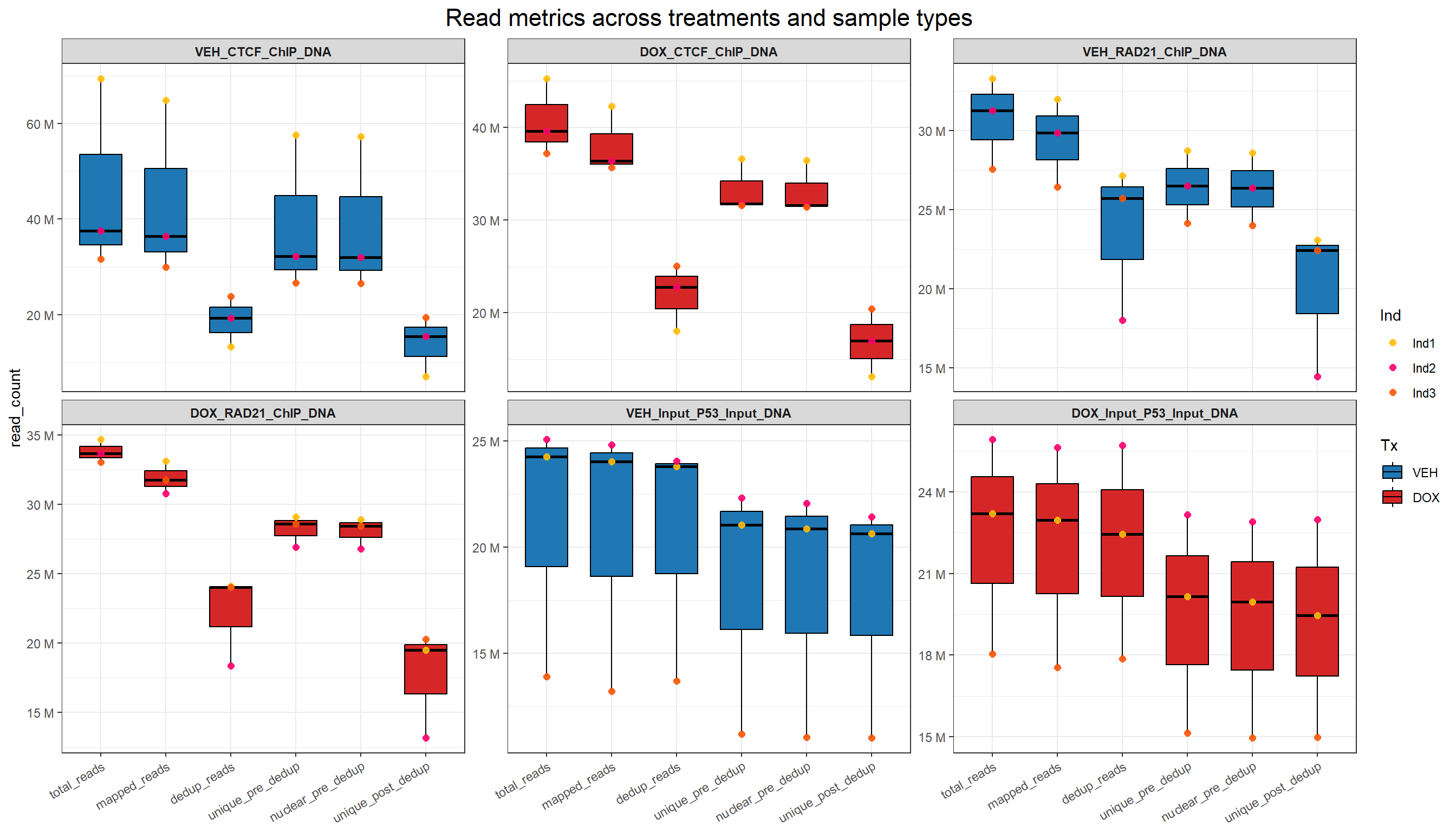
📌 Comparison of VEH and DOX reads across ChIP and Input samples
# ============================================================
# 📊 Comparison of VEH and DOX read metrics across ChIP/Input samples
# ============================================================

library(dplyr)
library(tidyr)
library(ggplot2)
library(scales)

# ---- Ensure numeric ----
map <- map %>%
  mutate(
    Total.Reads..before.trimming.              = as.numeric(Total.Reads..before.trimming.),
    Mapped.Reads                               = as.numeric(Mapped.Reads),
    Reads.after.deduplication                  = as.numeric(Reads.after.deduplication),
    Uniquely.mapped.reads.before.deduplication = as.numeric(Uniquely.mapped.reads.before.deduplication),
    Uniquely.mapped.reads.after.deduplication  = as.numeric(Uniquely.mapped.reads.after.deduplication)
  )

# ---- Metric definitions ----
metric_order <- c(
  "Total.Reads..before.trimming.",
  "Mapped.Reads",
  "Reads.after.deduplication",
  "Uniquely.mapped.reads.before.deduplication",
  "Uniquely.mapped.reads.after.deduplication"
)

metric_labels <- c(
  "Total.Reads..before.trimming."              = "total_reads",
  "Mapped.Reads"                               = "mapped_reads",
  "Reads.after.deduplication"                  = "dedup_reads",
  "Uniquely.mapped.reads.before.deduplication" = "unique_pre_dedup",
  "Uniquely.mapped.reads.after.deduplication"  = "unique_post_dedup"
)

# ---- Reshape ----
long5 <- map %>%
  dplyr::select(Ind, Type, Treatment, dplyr::all_of(metric_order)) %>%
  pivot_longer(
    cols = dplyr::all_of(metric_order),
    names_to = "Metric", values_to = "Reads"
  ) %>%
  mutate(
    Metric = factor(Metric, levels = metric_order, labels = metric_labels),
    Ind    = factor(Ind, levels = sort(unique(Ind))),
    Tx     = ifelse(grepl("^VEH", Treatment), "VEH", "DOX"),
    Tx     = factor(Tx, levels = c("VEH", "DOX")),
    # Build clean facet names: e.g. VEH_TOP2B_ChIP
    Facet  = paste(Tx, gsub("VEH_|DOX_", "", Treatment), Type, sep = "_"),
    Facet  = factor(Facet, levels = unique(paste(Tx, gsub("VEH_|DOX_", "", Treatment), Type, sep = "_")))
  ) %>%
  droplevels() %>%
  mutate(Reads = ifelse(Reads < 0, 0, Reads))  # Clamp negatives to 0

# ---- Colors ----
Ind_palc <- c("#ffbe0b","#ff006e","#fb5607","#8338ec","#3a86ff","#4a4e69")
tx_cols  <- c("VEH" = "#1f77b4", "DOX" = "#d62728")

# ---- Plot ----
ggplot(long5, aes(x = Metric, y = Reads)) +
  geom_boxplot(aes(fill = Tx),
               color = "black", width = 0.65, outlier.shape = NA,
               position = position_dodge(width = 0.75)) +
  geom_point(aes(color = Ind, group = Tx),
             position = position_dodge(width = 0.75),
             size = 2, alpha = 0.9) +
  scale_color_manual(values = Ind_palc, name = "Ind") +
  scale_fill_manual(values = tx_cols, name = "Tx") +
  scale_y_continuous(
    labels = label_number(suffix = " M", scale = 1e-6),
    expand = c(0, 0)
  ) +
  coord_cartesian(ylim = c(0, NA)) +  # Force y-axis start from 0
  facet_wrap(~Facet, scales = "free_y", ncol = 3) +
  labs(
    title = "Read metrics across treatments and sample types",
    x = NULL,
    y = "read_count"
  ) +
  theme_bw() +
  theme(
    plot.title   = element_text(size = rel(1.5), hjust = 0.5),
    axis.text.x  = element_text(angle = 30, hjust = 1),
    strip.text.x = element_text(face = "bold"),
    panel.grid.minor = element_blank()
  )
sessionInfo()R version 4.3.0 (2023-04-21 ucrt)
Platform: x86_64-w64-mingw32/x64 (64-bit)
Running under: Windows 11 x64 (build 26100)
Matrix products: default
locale:
[1] LC_COLLATE=English_United States.utf8
[2] LC_CTYPE=English_United States.utf8
[3] LC_MONETARY=English_United States.utf8
[4] LC_NUMERIC=C
[5] LC_TIME=English_United States.utf8
time zone: America/Chicago
tzcode source: internal
attached base packages:
[1] stats graphics grDevices utils datasets methods base
other attached packages:
[1] ggpubr_0.6.0 Hmisc_5.2-3 corrplot_0.95 ggrepel_0.9.6
[5] cowplot_1.1.3 biomaRt_2.58.2 scales_1.3.0 lubridate_1.9.4
[9] forcats_1.0.0 stringr_1.5.1 dplyr_1.1.4 purrr_1.0.4
[13] readr_2.1.5 tidyr_1.3.1 tibble_3.2.1 ggplot2_3.5.2
[17] tidyverse_2.0.0 data.table_1.17.0 reshape2_1.4.4 gridExtra_2.3
[21] RColorBrewer_1.1-3 edgeR_4.0.16 limma_3.58.1
loaded via a namespace (and not attached):
[1] DBI_1.2.3 bitops_1.0-9 rlang_1.1.3
[4] magrittr_2.0.3 git2r_0.36.2 compiler_4.3.0
[7] RSQLite_2.3.9 png_0.1-8 vctrs_0.6.5
[10] pkgconfig_2.0.3 crayon_1.5.3 fastmap_1.2.0
[13] backports_1.5.0 dbplyr_2.5.0 XVector_0.42.0
[16] labeling_0.4.3 promises_1.3.2 rmarkdown_2.29
[19] tzdb_0.5.0 bit_4.6.0 xfun_0.52
[22] zlibbioc_1.48.2 cachem_1.1.0 GenomeInfoDb_1.38.8
[25] jsonlite_2.0.0 progress_1.2.3 blob_1.2.4
[28] later_1.3.2 broom_1.0.8 prettyunits_1.2.0
[31] cluster_2.1.8.1 R6_2.6.1 bslib_0.9.0
[34] stringi_1.8.3 car_3.1-3 rpart_4.1.24
[37] jquerylib_0.1.4 Rcpp_1.0.12 knitr_1.50
[40] base64enc_0.1-3 IRanges_2.36.0 httpuv_1.6.15
[43] nnet_7.3-20 timechange_0.3.0 tidyselect_1.2.1
[46] abind_1.4-8 rstudioapi_0.17.1 yaml_2.3.10
[49] curl_6.2.2 lattice_0.22-7 plyr_1.8.9
[52] Biobase_2.62.0 withr_3.0.2 KEGGREST_1.42.0
[55] evaluate_1.0.3 foreign_0.8-90 BiocFileCache_2.10.2
[58] xml2_1.3.8 Biostrings_2.70.3 pillar_1.10.2
[61] filelock_1.0.3 carData_3.0-5 whisker_0.4.1
[64] checkmate_2.3.2 stats4_4.3.0 generics_0.1.3
[67] rprojroot_2.0.4 RCurl_1.98-1.17 S4Vectors_0.40.2
[70] hms_1.1.3 munsell_0.5.1 glue_1.7.0
[73] tools_4.3.0 ggsignif_0.6.4 locfit_1.5-9.12
[76] fs_1.6.3 XML_3.99-0.18 grid_4.3.0
[79] AnnotationDbi_1.64.1 colorspace_2.1-0 GenomeInfoDbData_1.2.11
[82] htmlTable_2.4.3 Formula_1.2-5 cli_3.6.1
[85] rappdirs_0.3.3 workflowr_1.7.1 gtable_0.3.6
[88] rstatix_0.7.2 sass_0.4.10 digest_0.6.34
[91] BiocGenerics_0.48.1 farver_2.1.2 htmlwidgets_1.6.4
[94] memoise_2.0.1 htmltools_0.5.8.1 lifecycle_1.0.4
[97] httr_1.4.7 statmod_1.5.0 bit64_4.6.0-1