Peak Calling cutoff (TOP2B and P53)
Last updated: 2025-09-01
Checks: 6 1
Knit directory: ChIPSeq_project/
This reproducible R Markdown analysis was created with workflowr (version 1.7.1). The Checks tab describes the reproducibility checks that were applied when the results were created. The Past versions tab lists the development history.
The R Markdown file has unstaged changes. To know which version of
the R Markdown file created these results, you’ll want to first commit
it to the Git repo. If you’re still working on the analysis, you can
ignore this warning. When you’re finished, you can run
wflow_publish to commit the R Markdown file and build the
HTML.
Great job! The global environment was empty. Objects defined in the global environment can affect the analysis in your R Markdown file in unknown ways. For reproduciblity it’s best to always run the code in an empty environment.
The command set.seed(20250815) was run prior to running
the code in the R Markdown file. Setting a seed ensures that any results
that rely on randomness, e.g. subsampling or permutations, are
reproducible.
Great job! Recording the operating system, R version, and package versions is critical for reproducibility.
Nice! There were no cached chunks for this analysis, so you can be confident that you successfully produced the results during this run.
Great job! Using relative paths to the files within your workflowr project makes it easier to run your code on other machines.
Great! You are using Git for version control. Tracking code development and connecting the code version to the results is critical for reproducibility.
The results in this page were generated with repository version bf6352f. See the Past versions tab to see a history of the changes made to the R Markdown and HTML files.
Note that you need to be careful to ensure that all relevant files for
the analysis have been committed to Git prior to generating the results
(you can use wflow_publish or
wflow_git_commit). workflowr only checks the R Markdown
file, but you know if there are other scripts or data files that it
depends on. Below is the status of the Git repository when the results
were generated:
Ignored files:
    Ignored:    .Rhistory
    Ignored:    .Rproj.user/

Untracked files:
    Untracked:  data/ELBOW_TOP2B_broad.csv
    Untracked:  data/ELBOW_TOP2B_narrow.csv
    Untracked:  data/macs3_broad_out_TOP2B/ELBOW_TOP2B_broad.csv
    Untracked:  data/macs3_broad_out_TOP2B/ELBOW_TOP2B_broad.xlsx
    Untracked:  data/macs3_broad_out_TOP2B/run_elbow_q.sh
    Untracked:  data/macs3_narrow_out_TOP2B/ELBOW_Q_SUMMARY.xlsx

Unstaged changes:
    Modified:   analysis/Peak_Calling_cutoff_TOP2B_P53.Rmd
Note that any generated files, e.g. HTML, png, CSS, etc., are not included in this status report because it is ok for generated content to have uncommitted changes.
These are the previous versions of the repository in which changes were
made to the R Markdown
(analysis/Peak_Calling_cutoff_TOP2B_P53.Rmd) and HTML
(docs/Peak_Calling_cutoff_TOP2B_P53.html) files. If you’ve
configured a remote Git repository (see ?wflow_git_remote),
click on the hyperlinks in the table below to view the files as they
were in that past version.
| File | Version | Author | Date | Message |
|---|---|---|---|---|
| html | 3cfce7f | sayanpaul01 | 2025-08-31 | Commit |
| Rmd | bc515e6 | sayanpaul01 | 2025-08-31 | Commit |
| html | bc515e6 | sayanpaul01 | 2025-08-31 | Commit |
| Rmd | 9c77a6c | sayanpaul01 | 2025-08-24 | Commit |
| html | 9c77a6c | sayanpaul01 | 2025-08-24 | Commit |
📌 TOP2B broad peaks (before deduplication)
library(tidyverse)Warning: package 'tidyverse' was built under R version 4.3.2Warning: package 'tidyr' was built under R version 4.3.3Warning: package 'readr' was built under R version 4.3.3Warning: package 'purrr' was built under R version 4.3.3Warning: package 'dplyr' was built under R version 4.3.2Warning: package 'stringr' was built under R version 4.3.2Warning: package 'lubridate' was built under R version 4.3.3── Attaching core tidyverse packages ──────────────────────── tidyverse 2.0.0 ──
✔ dplyr 1.1.4 ✔ readr 2.1.5
✔ forcats 1.0.0 ✔ stringr 1.5.1
✔ ggplot2 3.5.2 ✔ tibble 3.2.1
✔ lubridate 1.9.4 ✔ tidyr 1.3.1
✔ purrr 1.0.4
── Conflicts ────────────────────────────────────────── tidyverse_conflicts() ──
✖ dplyr::filter() masks stats::filter()
✖ dplyr::lag() masks stats::lag()
ℹ Use the conflicted package (<http://conflicted.r-lib.org/>) to force all conflicts to become errorslibrary(readr)
library(scales) # <- needed for label_number()Warning: package 'scales' was built under R version 4.3.2
Attaching package: 'scales'

The following object is masked from 'package:purrr':

    discard

The following object is masked from 'package:readr':

    col_factor
# --- metadata ---
metadata <- tribble(
~Sample, ~Sample_Det,
"MCW_SP_ChIP27", "Ind1_VEH_TOP2B",
"MCW_SP_ChIP28", "Ind1_DOX_TOP2B",
"MCW_SP_ChIP31", "Ind2_VEH_TOP2B",
"MCW_SP_ChIP32", "Ind2_DOX_TOP2B",
"MCW_SP_ChIP39", "Ind3_VEH_TOP2B",
"MCW_SP_ChIP40", "Ind3_DOX_TOP2B",
"MCW_SP_ChIP43", "Ind4_VEH_TOP2B",
"MCW_SP_ChIP44", "Ind4_DOX_TOP2B",
"MCW_SP_ChIP51", "Ind5_VEH_TOP2B",
"MCW_SP_ChIP52", "Ind5_DOX_TOP2B",
"MCW_SP_ChIP55", "Ind6_VEH_TOP2B",
"MCW_SP_ChIP56", "Ind6_DOX_TOP2B"
) |> mutate(
Sample = factor(Sample, levels = Sample),
Sample_Det = factor(Sample_Det, levels = Sample_Det)
)
# --- load all cutoff analysis files ---
files <- list.files("data/macs3_broad_out_TOP2B",
pattern = "_cutoff_analysis\\.txt$", full.names = TRUE)
df <- files |>
set_names() |>
map_dfr(~ read_delim(.x, delim = "\t", show_col_types = FALSE), .id = "filepath") |>
mutate(Sample = basename(filepath) |> str_remove("_cutoff_analysis\\.txt")) |>
left_join(metadata, by = "Sample") |>
mutate(Sample_Det = factor(Sample_Det, levels = levels(metadata$Sample_Det))) |>
arrange(Sample_Det, qscore)
# Common x-scale (guarantees tick at 0)
x_fixed <- scale_x_continuous(
limits = c(0, 7),
breaks = 0:7,
labels = as.character(0:7),
expand = c(0, 0)
)
# ---- Plot with linear y-axis ----
p_linear <- ggplot(df, aes(qscore, npeaks, group = Sample)) +
geom_line(size = 0.8, color = "#d95f02") +
facet_wrap(~ Sample_Det, scales = "free_y", ncol = 6) +
x_fixed +
scale_y_continuous(labels = scales::label_number(big.mark = ",")) +
labs(x = "Q Score", y = "Peak Counts (linear)") +
theme_minimal(base_size = 12) +
theme(strip.text = element_text(face = "bold", size = 10),
panel.grid.minor = element_blank())Warning: Using `size` aesthetic for lines was deprecated in ggplot2 3.4.0.
ℹ Please use `linewidth` instead.
This warning is displayed once every 8 hours.
Call `lifecycle::last_lifecycle_warnings()` to see where this warning was
generated.# ---- Plot with log10 y-axis ----
p_log <- df |>
mutate(npeaks = ifelse(npeaks <= 0, NA, npeaks)) |>
ggplot(aes(qscore, npeaks, group = Sample)) +
geom_line(size = 0.8, color = "#d95f02") +
facet_wrap(~ Sample_Det, scales = "free_y", ncol = 6) +
x_fixed +
scale_y_log10(labels = scales::label_number(big.mark = ",")) +
labs(x = "Q Score", y = "Peak Counts (log10)") +
theme_minimal(base_size = 12) +
theme(strip.text = element_text(face = "bold", size = 10),
panel.grid.minor = element_blank())
# ---- Print both ----
p_linear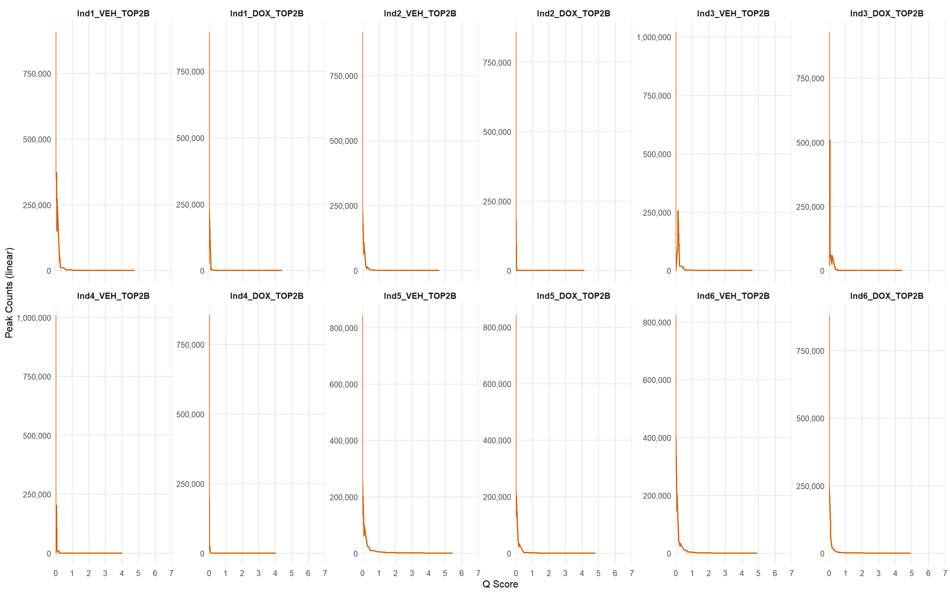
| Version | Author | Date |
|---|---|---|
| 9c77a6c | sayanpaul01 | 2025-08-24 |
p_log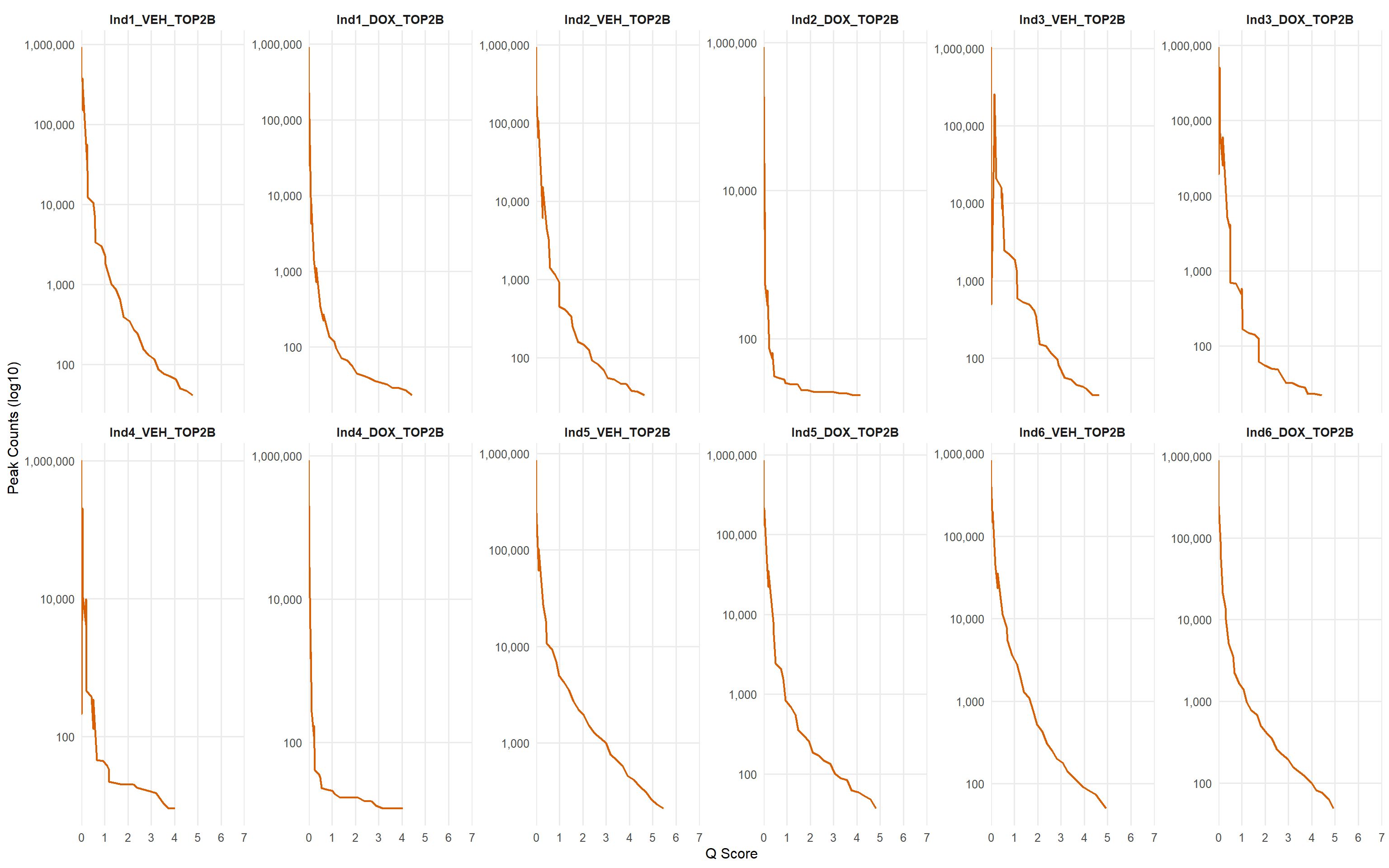
| Version | Author | Date |
|---|---|---|
| 9c77a6c | sayanpaul01 | 2025-08-24 |
📌 TOP2B narrow peaks (before deduplication)
library(tidyverse)
library(readr)

# --- metadata ---
metadata <- tribble(
  ~Sample,           ~Sample_Det,
  "MCW_SP_ChIP27",   "Ind1_VEH_TOP2B",
  "MCW_SP_ChIP28",   "Ind1_DOX_TOP2B",
  "MCW_SP_ChIP31",   "Ind2_VEH_TOP2B",
  "MCW_SP_ChIP32",   "Ind2_DOX_TOP2B",
  "MCW_SP_ChIP39",   "Ind3_VEH_TOP2B",
  "MCW_SP_ChIP40",   "Ind3_DOX_TOP2B",
  "MCW_SP_ChIP43",   "Ind4_VEH_TOP2B",
  "MCW_SP_ChIP44",   "Ind4_DOX_TOP2B",
  "MCW_SP_ChIP51",   "Ind5_VEH_TOP2B",
  "MCW_SP_ChIP52",   "Ind5_DOX_TOP2B",
  "MCW_SP_ChIP55",   "Ind6_VEH_TOP2B",
  "MCW_SP_ChIP56",   "Ind6_DOX_TOP2B"
)

# --- load all cutoff analysis files ---
files <- list.files("data/macs3_narrow_out_TOP2B", pattern = "_cutoff_analysis\\.txt$", full.names = TRUE)

df <- files %>%
  set_names() %>%
  map_dfr(~ read_delim(.x, delim = "\t", show_col_types = FALSE), .id = "filepath") %>%
  mutate(Sample = basename(filepath) %>% str_remove("_cutoff_analysis\\.txt")) %>%
  left_join(metadata, by = "Sample")

# ---- Plot with linear y-axis ----
p_linear <- df %>%
  ggplot(aes(x = qscore, y = npeaks, group = Sample)) +
  geom_line(size = 0.8, color = "#d95f02") +
  facet_wrap(~ Sample_Det, scales = "free_y", ncol = 6) +
  scale_x_continuous(
    limits = c(0, 7),
    breaks = 0:7,
    labels = as.character(0:7),   # ensures "0" shows up
    expand = c(0, 0)
  ) +
  scale_y_continuous(labels = label_number(big.mark = ",")) +
  labs(x = "Q Score", y = "Peak Counts (linear)") +
  theme_minimal(base_size = 12) +
  theme(
    strip.text = element_text(face = "bold", size = 10),
    panel.grid.minor = element_blank()
  )

# ---- Plot with log10 y-axis ----
p_log <- df %>%
  ggplot(aes(x = qscore, y = npeaks, group = Sample)) +
  geom_line(size = 0.8, color = "#d95f02") +
  facet_wrap(~ Sample_Det, scales = "free_y", ncol = 6) +
  scale_x_continuous(
    limits = c(0, 7),
    breaks = 0:7,
    labels = as.character(0:7),
    expand = c(0, 0)
  ) +
  scale_y_log10(labels = label_number(big.mark = ",")) +
  labs(x = "Q Score", y = "Peak Counts (log10)") +
  theme_minimal(base_size = 12) +
  theme(
    strip.text = element_text(face = "bold", size = 10),
    panel.grid.minor = element_blank()
  )

# ---- Print both ----
p_linear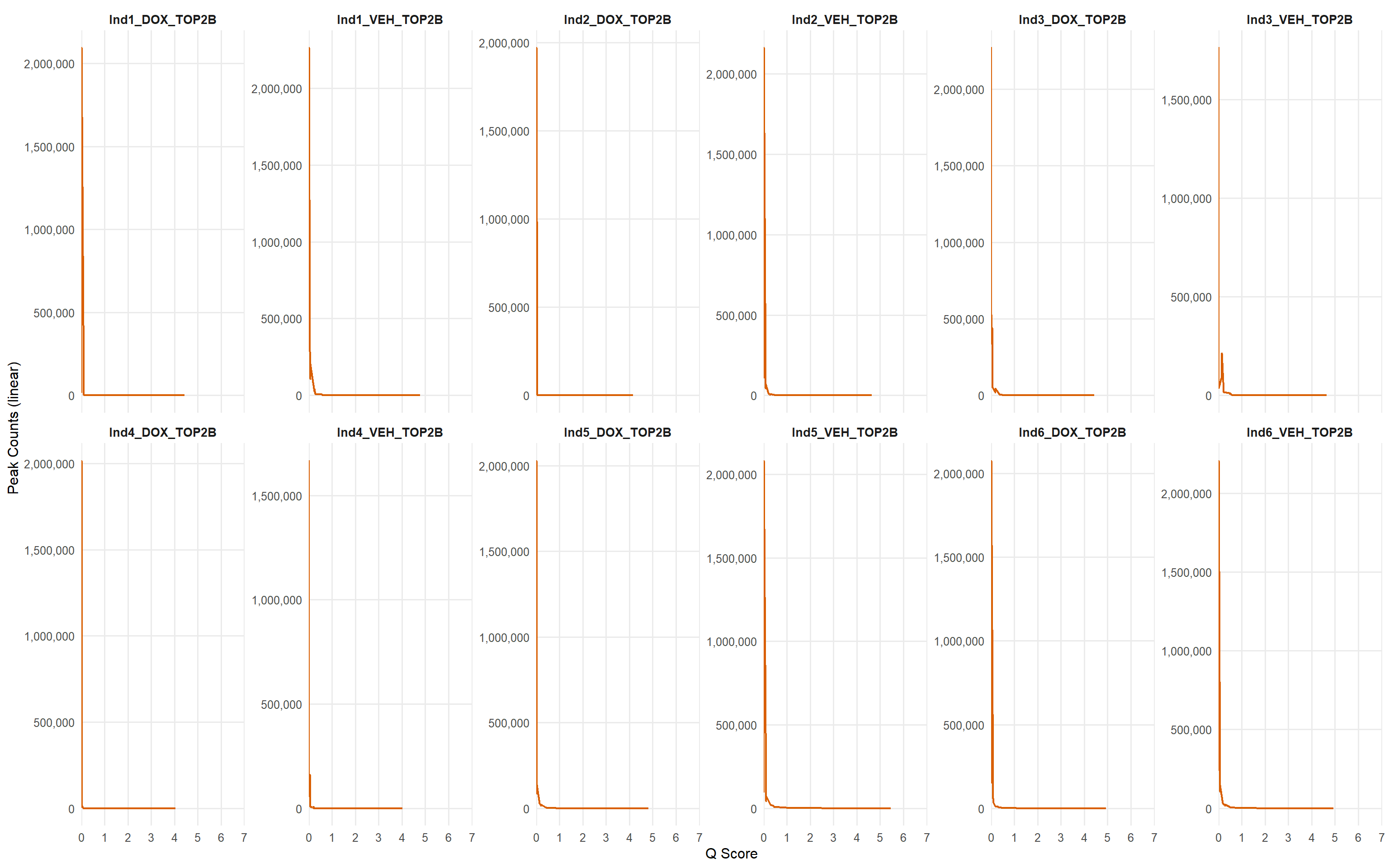
| Version | Author | Date |
|---|---|---|
| 9c77a6c | sayanpaul01 | 2025-08-24 |
p_log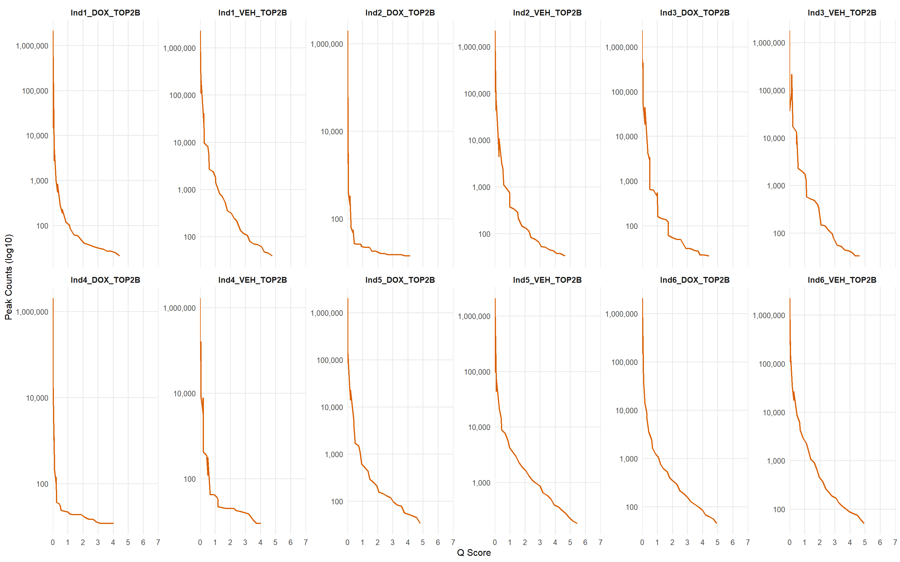
| Version | Author | Date |
|---|---|---|
| 9c77a6c | sayanpaul01 | 2025-08-24 |
📌 P53 narrow peaks (before deduplication)
library(tidyverse)
library(readr)
library(scales)

# --- metadata for p53 ---
metadata_p53 <- tribble(
  ~Sample,           ~Sample_Det,
  "MCW_SP_ChIP29",   "Ind1_VEH_p53",
  "MCW_SP_ChIP30",   "Ind1_DOX_p53",
  "MCW_SP_ChIP33",   "Ind2_VEH_p53",
  "MCW_SP_ChIP34",   "Ind2_DOX_p53",
  "MCW_SP_ChIP41",   "Ind3_VEH_p53",
  "MCW_SP_ChIP42",   "Ind3_DOX_p53",
  "MCW_SP_ChIP45",   "Ind4_VEH_p53",
  "MCW_SP_ChIP46",   "Ind4_DOX_p53",
  "MCW_SP_ChIP53",   "Ind5_VEH_p53",
  "MCW_SP_ChIP54",   "Ind5_DOX_p53",
  "MCW_SP_ChIP57",   "Ind6_VEH_p53",
  "MCW_SP_ChIP58",   "Ind6_DOX_p53"
) %>%
  mutate(
    Sample     = factor(Sample,     levels = Sample),
    Sample_Det = factor(Sample_Det, levels = Sample_Det)
  )

# --- load all cutoff-analysis files (edit path if needed) ---
data_dir <- "data/macs3_narrow_out_P53"   # <— change if your folder name differs
files <- list.files(data_dir, pattern = "_cutoff_analysis\\.txt$", full.names = TRUE)

df_p53 <- files %>%
  set_names() %>%
  map_dfr(~ read_delim(.x, delim = "\t", show_col_types = FALSE), .id = "filepath") %>%
  mutate(Sample = basename(filepath) %>% str_remove("_cutoff_analysis\\.txt")) %>%
  left_join(metadata_p53, by = "Sample") %>%
  mutate(Sample_Det = factor(Sample_Det, levels = levels(metadata_p53$Sample_Det))) %>%
  arrange(Sample_Det, qscore)

# --------- common x scale (forces 0..7 with a printed 0) ----------
x_fixed <- scale_x_continuous(
  limits = c(0, 7),
  breaks = 0:7,
  labels = as.character(0:7),
  expand = c(0, 0)
)

# ---- linear y ----
p_linear_p53 <- ggplot(df_p53, aes(qscore, npeaks, group = Sample)) +
  geom_line(size = 0.8, color = "#d95f02") +
  facet_wrap(~ Sample_Det, scales = "free_y", ncol = 6) +
  x_fixed +
  scale_y_continuous(labels = label_number(big.mark = ",")) +
  labs(x = "Q Score", y = "Peak Counts (linear)") +
  theme_minimal(base_size = 12) +
  theme(
    strip.text = element_text(face = "bold", size = 10),
    panel.grid.minor = element_blank()
  )

# ---- log10 y ----
p_log_p53 <- ggplot(df_p53, aes(qscore, npeaks, group = Sample)) +
  geom_line(size = 0.8, color = "#d95f02") +
  facet_wrap(~ Sample_Det, scales = "free_y", ncol = 6) +
  x_fixed +
  scale_y_log10(labels = label_number(big.mark = ",")) +
  labs(x = "Q Score", y = "Peak Counts (log10)") +
  theme_minimal(base_size = 12) +
  theme(
    strip.text = element_text(face = "bold", size = 10),
    panel.grid.minor = element_blank()
  )

# ---- show both ----
p_linear_p53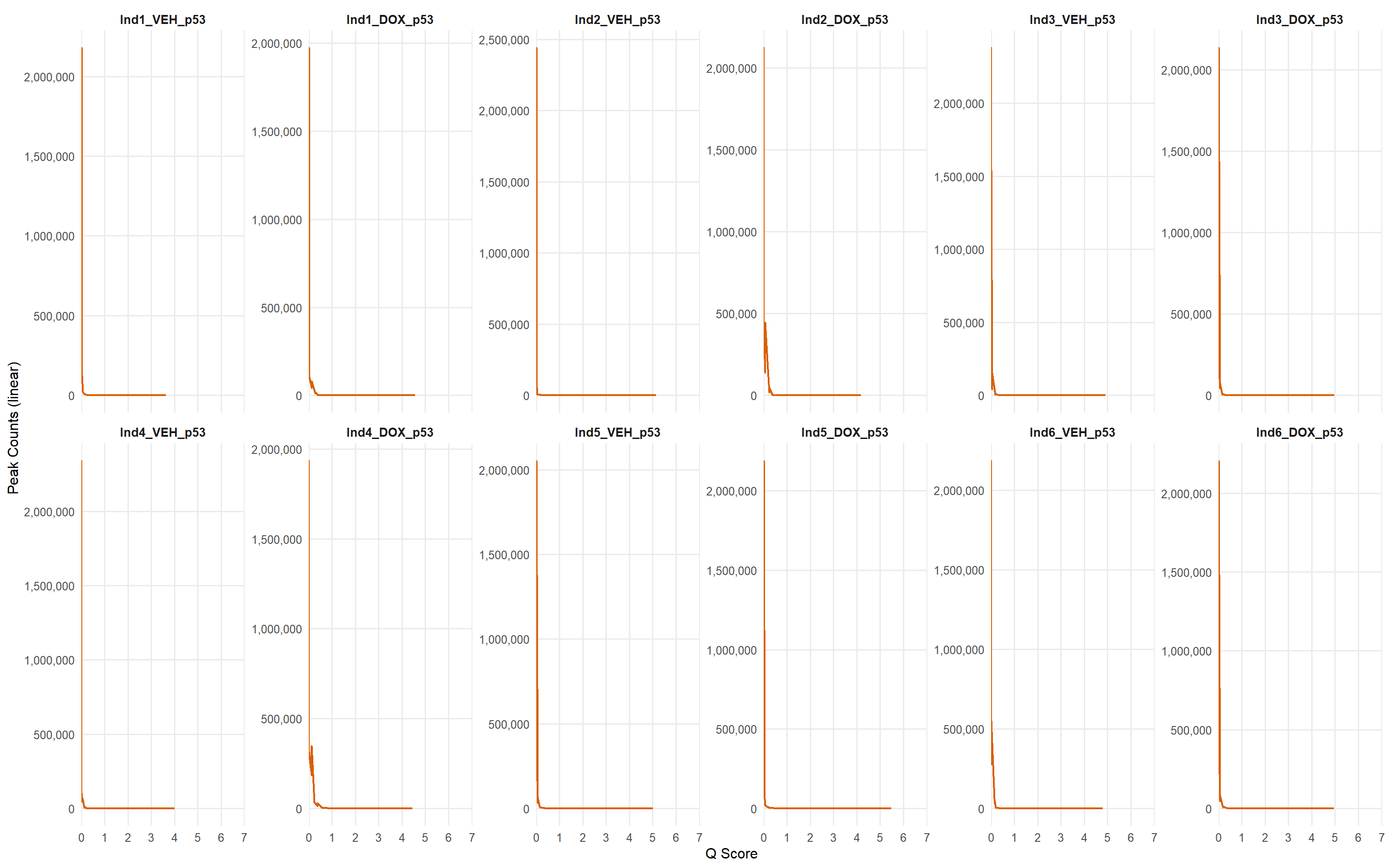
| Version | Author | Date |
|---|---|---|
| 9c77a6c | sayanpaul01 | 2025-08-24 |
p_log_p53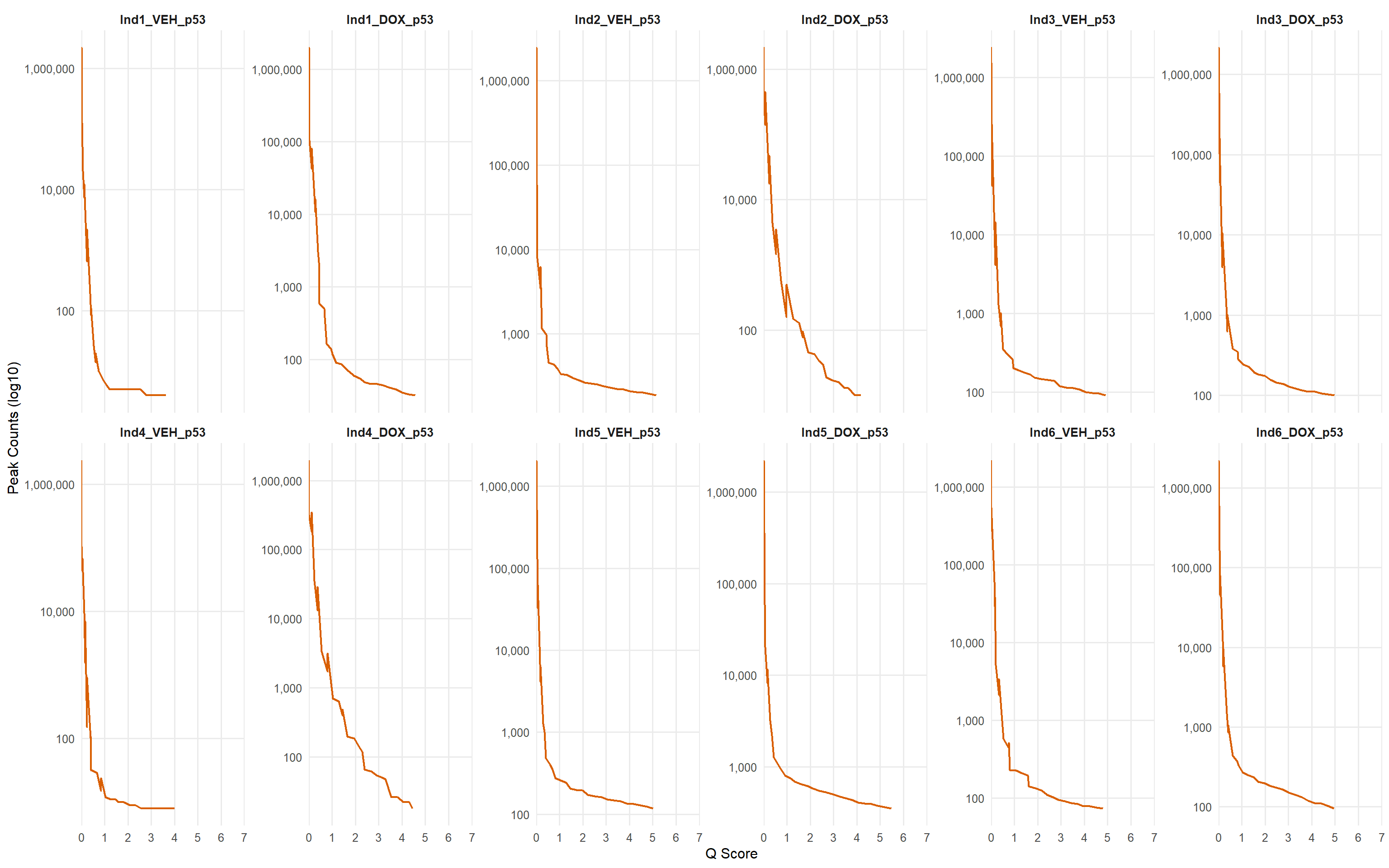
| Version | Author | Date |
|---|---|---|
| 9c77a6c | sayanpaul01 | 2025-08-24 |
📌 TOP2B broad peaks (after deduplication)
library(tidyverse)
library(readr)

# --- metadata ---
metadata <- tribble(
  ~Sample,           ~Sample_Det,
  "MCW_SP_ChIP27",   "Ind1_VEH_TOP2B",
  "MCW_SP_ChIP28",   "Ind1_DOX_TOP2B",
  "MCW_SP_ChIP31",   "Ind2_VEH_TOP2B",
  "MCW_SP_ChIP32",   "Ind2_DOX_TOP2B",
  "MCW_SP_ChIP39",   "Ind3_VEH_TOP2B",
  "MCW_SP_ChIP40",   "Ind3_DOX_TOP2B",
  "MCW_SP_ChIP43",   "Ind4_VEH_TOP2B",
  "MCW_SP_ChIP44",   "Ind4_DOX_TOP2B",
  "MCW_SP_ChIP51",   "Ind5_VEH_TOP2B",
  "MCW_SP_ChIP52",   "Ind5_DOX_TOP2B",
  "MCW_SP_ChIP55",   "Ind6_VEH_TOP2B",
  "MCW_SP_ChIP56",   "Ind6_DOX_TOP2B"
)

# --- load all cutoff analysis files ---
files <- list.files("data/macs3_broad_out_TOP2B_dedup", pattern = "_cutoff_analysis\\.txt$", full.names = TRUE)

df <- files %>%
  set_names() %>%
  map_dfr(~ read_delim(.x, delim = "\t", show_col_types = FALSE), .id = "filepath") %>%
  mutate(Sample = basename(filepath) %>% str_remove("_cutoff_analysis\\.txt")) %>%
  left_join(metadata, by = "Sample")

# ---- Plot with linear y-axis ----
p_linear <- df %>%
  ggplot(aes(x = qscore, y = npeaks, group = Sample)) +
  geom_line(size = 0.8, color = "#d95f02") +
  facet_wrap(~ Sample_Det, scales = "free_y", ncol = 6) +
  scale_x_continuous(
    limits = c(0, 7),
    breaks = 0:7,
    labels = as.character(0:7),   # ensures "0" shows up
    expand = c(0, 0)
  ) +
  scale_y_continuous(labels = label_number(big.mark = ",")) +
  labs(x = "Q Score", y = "Peak Counts (linear)") +
  theme_minimal(base_size = 12) +
  theme(
    strip.text = element_text(face = "bold", size = 10),
    panel.grid.minor = element_blank()
  )

# ---- Plot with log10 y-axis ----
p_log <- df %>%
  ggplot(aes(x = qscore, y = npeaks, group = Sample)) +
  geom_line(size = 0.8, color = "#d95f02") +
  facet_wrap(~ Sample_Det, scales = "free_y", ncol = 6) +
  scale_x_continuous(
    limits = c(0, 7),
    breaks = 0:7,
    labels = as.character(0:7),
    expand = c(0, 0)
  ) +
  scale_y_log10(labels = label_number(big.mark = ",")) +
  labs(x = "Q Score", y = "Peak Counts (log10)") +
  theme_minimal(base_size = 12) +
  theme(
    strip.text = element_text(face = "bold", size = 10),
    panel.grid.minor = element_blank()
  )

# ---- Print both ----
p_linear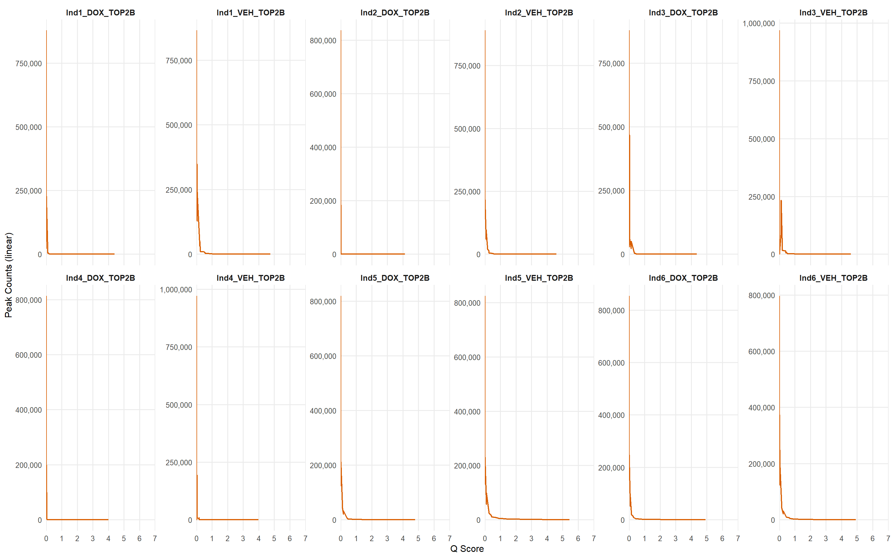
| Version | Author | Date |
|---|---|---|
| 9c77a6c | sayanpaul01 | 2025-08-24 |
p_log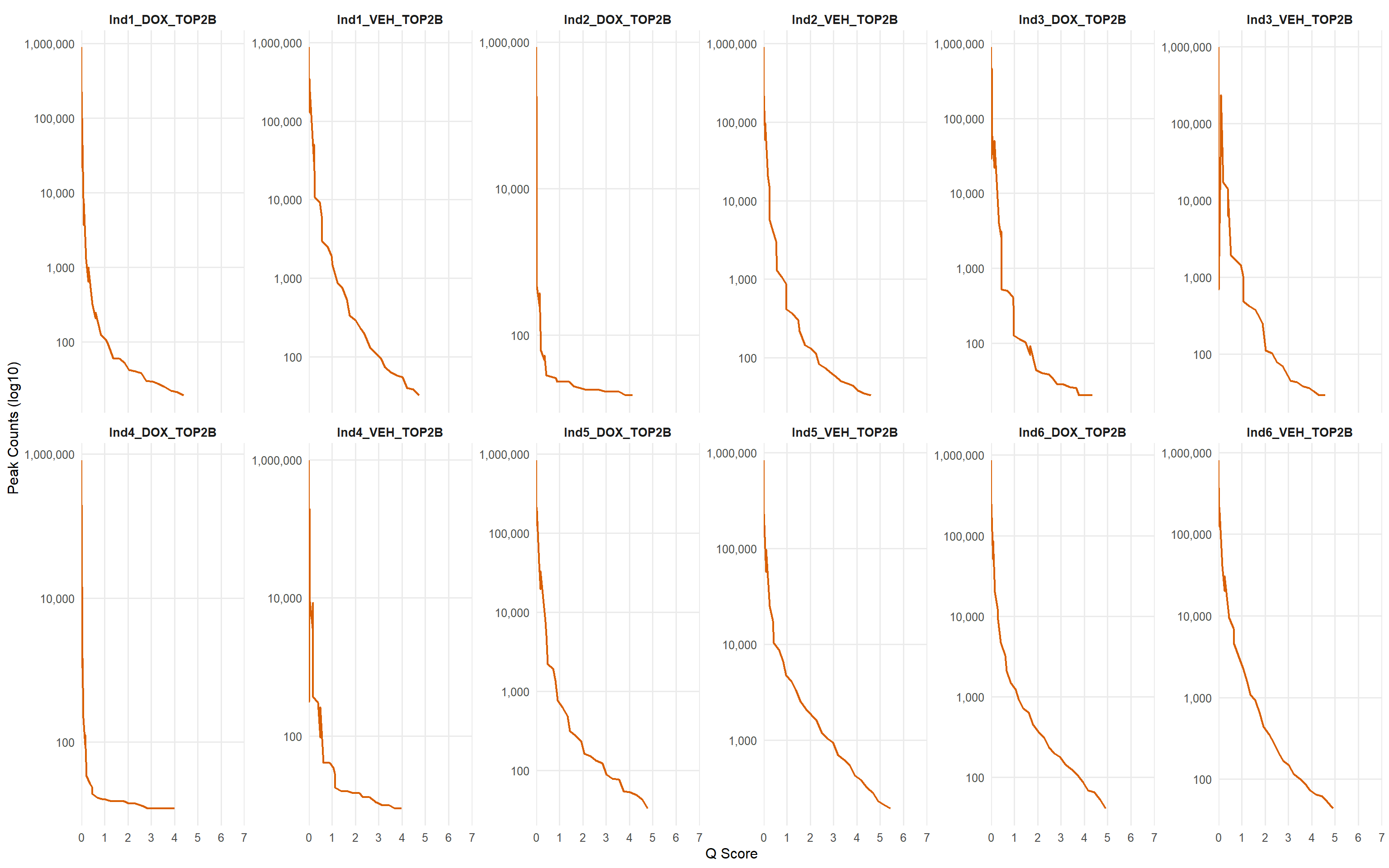
| Version | Author | Date |
|---|---|---|
| 9c77a6c | sayanpaul01 | 2025-08-24 |
📌 TOP2B narrow peaks (after deduplication)
library(tidyverse)
library(readr)

# --- metadata ---
metadata <- tribble(
  ~Sample,           ~Sample_Det,
  "MCW_SP_ChIP27",   "Ind1_VEH_TOP2B",
  "MCW_SP_ChIP28",   "Ind1_DOX_TOP2B",
  "MCW_SP_ChIP31",   "Ind2_VEH_TOP2B",
  "MCW_SP_ChIP32",   "Ind2_DOX_TOP2B",
  "MCW_SP_ChIP39",   "Ind3_VEH_TOP2B",
  "MCW_SP_ChIP40",   "Ind3_DOX_TOP2B",
  "MCW_SP_ChIP43",   "Ind4_VEH_TOP2B",
  "MCW_SP_ChIP44",   "Ind4_DOX_TOP2B",
  "MCW_SP_ChIP51",   "Ind5_VEH_TOP2B",
  "MCW_SP_ChIP52",   "Ind5_DOX_TOP2B",
  "MCW_SP_ChIP55",   "Ind6_VEH_TOP2B",
  "MCW_SP_ChIP56",   "Ind6_DOX_TOP2B"
)

# --- load all cutoff analysis files ---
files <- list.files("data/macs3_narrow_out_TOP2B_dedup", pattern = "_cutoff_analysis\\.txt$", full.names = TRUE)

df <- files %>%
  set_names() %>%
  map_dfr(~ read_delim(.x, delim = "\t", show_col_types = FALSE), .id = "filepath") %>%
  mutate(Sample = basename(filepath) %>% str_remove("_cutoff_analysis\\.txt")) %>%
  left_join(metadata, by = "Sample")

# ---- Plot with linear y-axis ----
p_linear <- df %>%
  ggplot(aes(x = qscore, y = npeaks, group = Sample)) +
  geom_line(size = 0.8, color = "#d95f02") +
  facet_wrap(~ Sample_Det, scales = "free_y", ncol = 6) +
  scale_x_continuous(
    limits = c(0, 7),
    breaks = 0:7,
    labels = as.character(0:7),   # ensures "0" shows up
    expand = c(0, 0)
  ) +
  scale_y_continuous(labels = label_number(big.mark = ",")) +
  labs(x = "Q Score", y = "Peak Counts (linear)") +
  theme_minimal(base_size = 12) +
  theme(
    strip.text = element_text(face = "bold", size = 10),
    panel.grid.minor = element_blank()
  )

# ---- Plot with log10 y-axis ----
p_log <- df %>%
  ggplot(aes(x = qscore, y = npeaks, group = Sample)) +
  geom_line(size = 0.8, color = "#d95f02") +
  facet_wrap(~ Sample_Det, scales = "free_y", ncol = 6) +
  scale_x_continuous(
    limits = c(0, 7),
    breaks = 0:7,
    labels = as.character(0:7),
    expand = c(0, 0)
  ) +
  scale_y_log10(labels = label_number(big.mark = ",")) +
  labs(x = "Q Score", y = "Peak Counts (log10)") +
  theme_minimal(base_size = 12) +
  theme(
    strip.text = element_text(face = "bold", size = 10),
    panel.grid.minor = element_blank()
  )

# ---- Print both ----
p_linear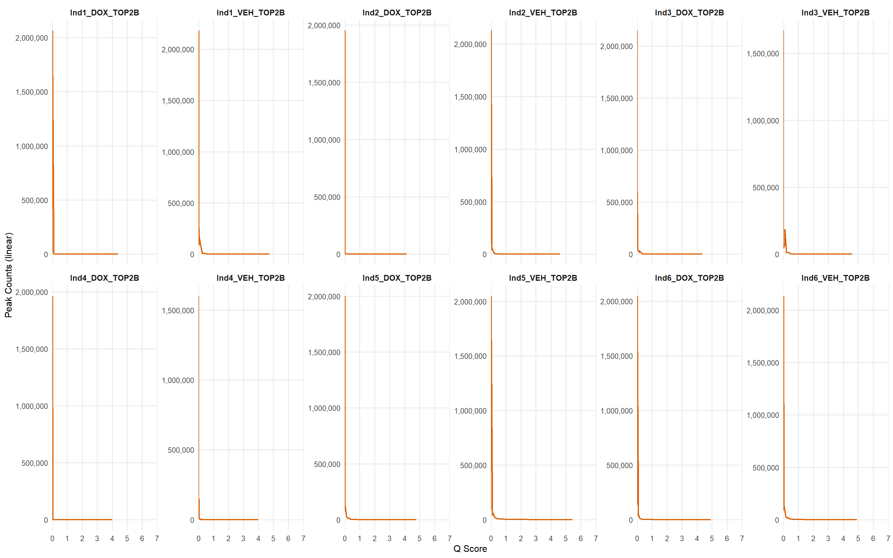
| Version | Author | Date |
|---|---|---|
| 9c77a6c | sayanpaul01 | 2025-08-24 |
p_log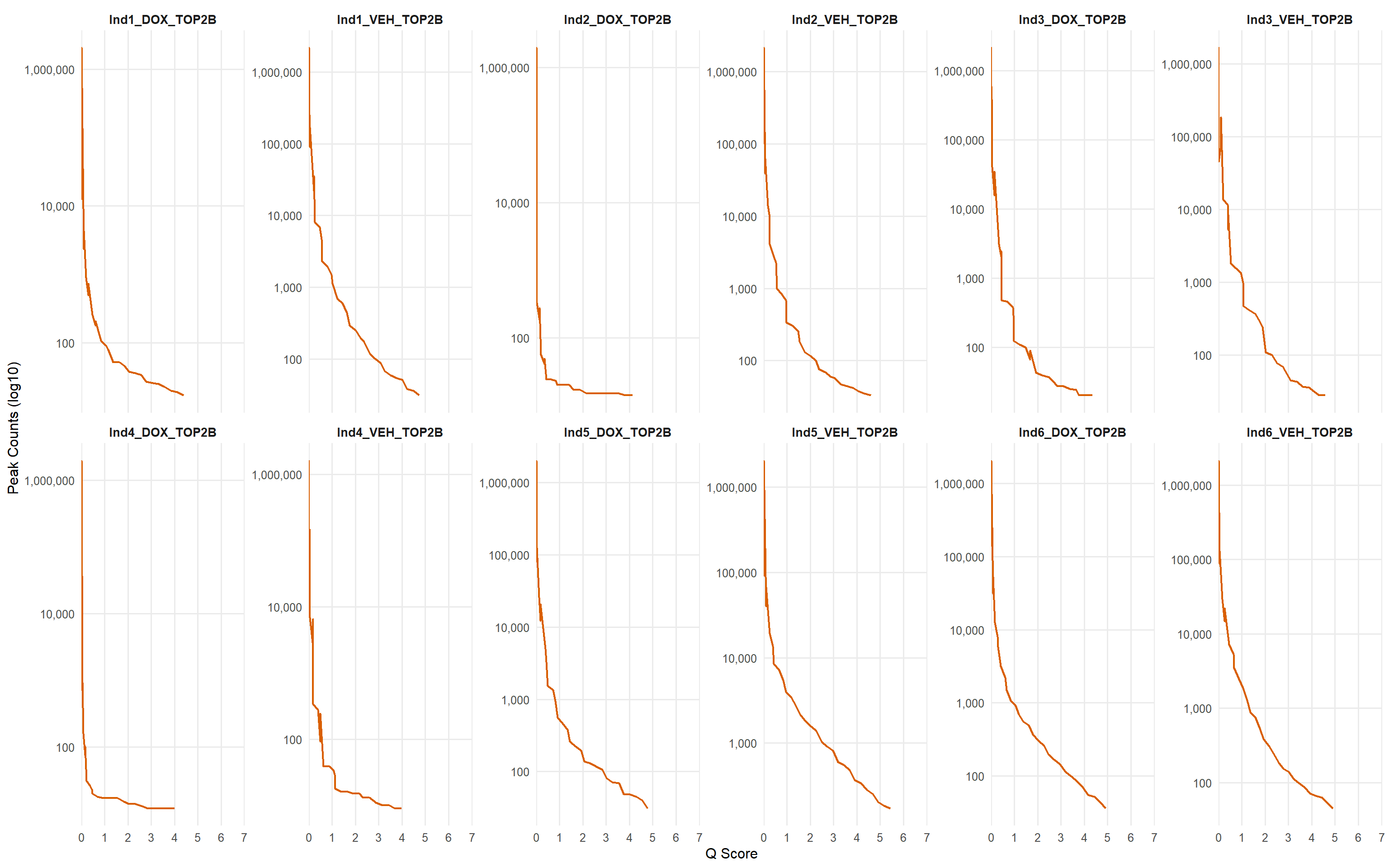
| Version | Author | Date |
|---|---|---|
| 9c77a6c | sayanpaul01 | 2025-08-24 |
📌 P53 narrow peaks (after deduplication)
library(tidyverse)
library(readr)
library(scales)

# --- metadata for p53 ---
metadata_p53 <- tribble(
  ~Sample,           ~Sample_Det,
  "MCW_SP_ChIP29",   "Ind1_VEH_p53",
  "MCW_SP_ChIP30",   "Ind1_DOX_p53",
  "MCW_SP_ChIP33",   "Ind2_VEH_p53",
  "MCW_SP_ChIP34",   "Ind2_DOX_p53",
  "MCW_SP_ChIP41",   "Ind3_VEH_p53",
  "MCW_SP_ChIP42",   "Ind3_DOX_p53",
  "MCW_SP_ChIP45",   "Ind4_VEH_p53",
  "MCW_SP_ChIP46",   "Ind4_DOX_p53",
  "MCW_SP_ChIP53",   "Ind5_VEH_p53",
  "MCW_SP_ChIP54",   "Ind5_DOX_p53",
  "MCW_SP_ChIP57",   "Ind6_VEH_p53",
  "MCW_SP_ChIP58",   "Ind6_DOX_p53"
) %>%
  mutate(
    Sample     = factor(Sample,     levels = Sample),
    Sample_Det = factor(Sample_Det, levels = Sample_Det)
  )

# --- load all cutoff-analysis files (edit path if needed) ---
data_dir <- "data/macs3_narrow_out_P53_dedup"   # <— change if your folder name differs
files <- list.files(data_dir, pattern = "_cutoff_analysis\\.txt$", full.names = TRUE)

df_p53 <- files %>%
  set_names() %>%
  map_dfr(~ read_delim(.x, delim = "\t", show_col_types = FALSE), .id = "filepath") %>%
  mutate(Sample = basename(filepath) %>% str_remove("_cutoff_analysis\\.txt")) %>%
  left_join(metadata_p53, by = "Sample") %>%
  mutate(Sample_Det = factor(Sample_Det, levels = levels(metadata_p53$Sample_Det))) %>%
  arrange(Sample_Det, qscore)

# --------- common x scale (forces 0..7 with a printed 0) ----------
x_fixed <- scale_x_continuous(
  limits = c(0, 7),
  breaks = 0:7,
  labels = as.character(0:7),
  expand = c(0, 0)
)

# ---- linear y ----
p_linear_p53 <- ggplot(df_p53, aes(qscore, npeaks, group = Sample)) +
  geom_line(size = 0.8, color = "#d95f02") +
  facet_wrap(~ Sample_Det, scales = "free_y", ncol = 6) +
  x_fixed +
  scale_y_continuous(labels = label_number(big.mark = ",")) +
  labs(x = "Q Score", y = "Peak Counts (linear)") +
  theme_minimal(base_size = 12) +
  theme(
    strip.text = element_text(face = "bold", size = 10),
    panel.grid.minor = element_blank()
  )

# ---- log10 y ----
p_log_p53 <- ggplot(df_p53, aes(qscore, npeaks, group = Sample)) +
  geom_line(size = 0.8, color = "#d95f02") +
  facet_wrap(~ Sample_Det, scales = "free_y", ncol = 6) +
  x_fixed +
  scale_y_log10(labels = label_number(big.mark = ",")) +
  labs(x = "Q Score", y = "Peak Counts (log10)") +
  theme_minimal(base_size = 12) +
  theme(
    strip.text = element_text(face = "bold", size = 10),
    panel.grid.minor = element_blank()
  )

# ---- show both ----
p_linear_p53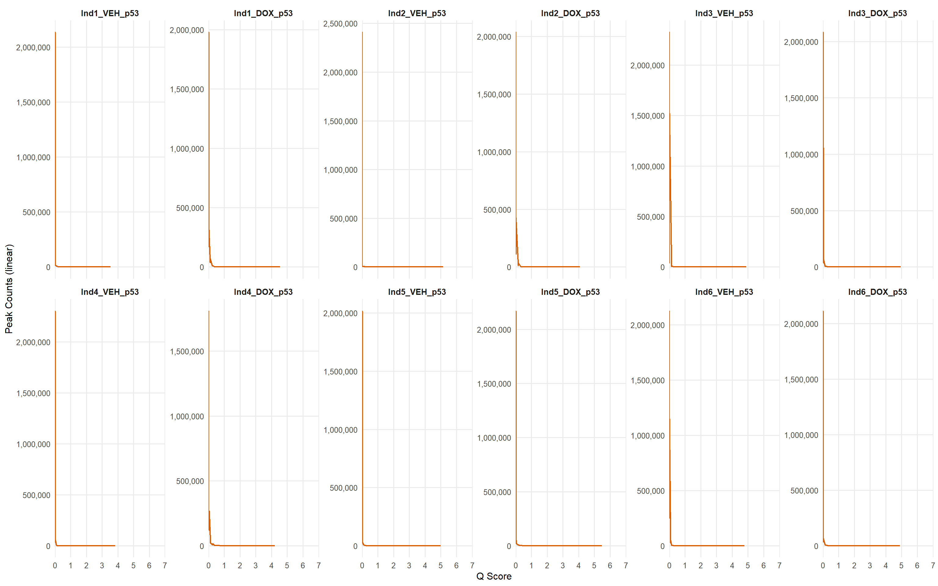
| Version | Author | Date |
|---|---|---|
| 9c77a6c | sayanpaul01 | 2025-08-24 |
p_log_p53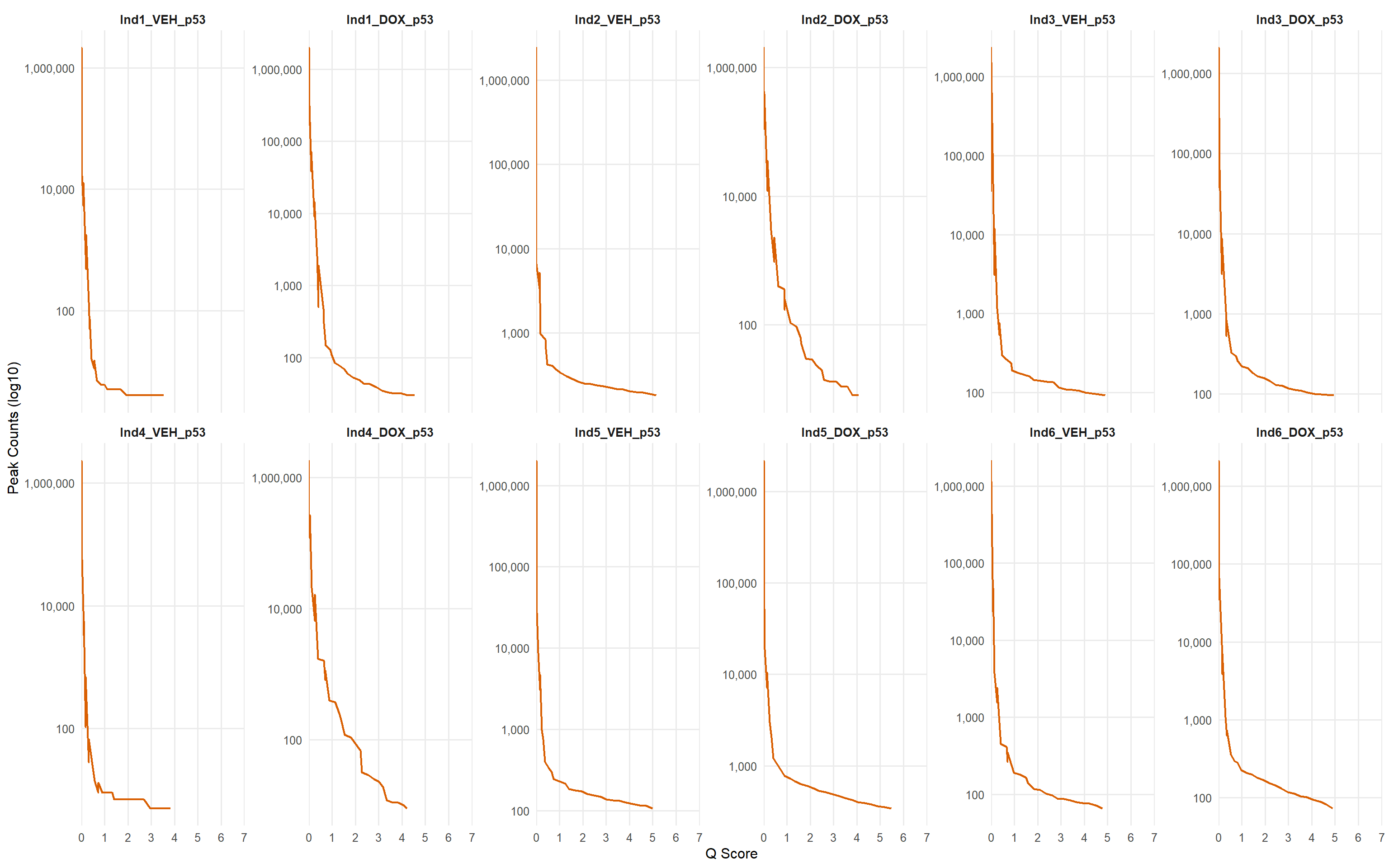
| Version | Author | Date |
|---|---|---|
| 9c77a6c | sayanpaul01 | 2025-08-24 |
📌 TOP2B broad peaks length (before deduplication)
library(tidyverse)
library(readr)
library(scales)

# --- metadata ---
metadata <- tribble(
  ~Sample,           ~Sample_Det,
  "MCW_SP_ChIP27",   "Ind1_VEH_TOP2B",
  "MCW_SP_ChIP28",   "Ind1_DOX_TOP2B",
  "MCW_SP_ChIP31",   "Ind2_VEH_TOP2B",
  "MCW_SP_ChIP32",   "Ind2_DOX_TOP2B",
  "MCW_SP_ChIP39",   "Ind3_VEH_TOP2B",
  "MCW_SP_ChIP40",   "Ind3_DOX_TOP2B",
  "MCW_SP_ChIP43",   "Ind4_VEH_TOP2B",
  "MCW_SP_ChIP44",   "Ind4_DOX_TOP2B",
  "MCW_SP_ChIP51",   "Ind5_VEH_TOP2B",
  "MCW_SP_ChIP52",   "Ind5_DOX_TOP2B",
  "MCW_SP_ChIP55",   "Ind6_VEH_TOP2B",
  "MCW_SP_ChIP56",   "Ind6_DOX_TOP2B"
) |> mutate(
  Sample     = factor(Sample,     levels = Sample),
  Sample_Det = factor(Sample_Det, levels = Sample_Det)
)

# --- load all cutoff analysis files ---
files <- list.files("data/macs3_broad_out_TOP2B",
                    pattern = "_cutoff_analysis\\.txt$", full.names = TRUE)

df <- files |>
  set_names() |>
  map_dfr(~ read_delim(.x, delim = "\t", show_col_types = FALSE), .id = "filepath") |>
  mutate(Sample = basename(filepath) |> str_remove("_cutoff_analysis\\.txt")) |>
  left_join(metadata, by = "Sample") |>
  mutate(Sample_Det = factor(Sample_Det, levels = levels(metadata$Sample_Det))) |>
  arrange(Sample_Det, qscore)

# Common x-scale (guarantees tick at 0)
x_fixed <- scale_x_continuous(
  limits = c(0, 7),
  breaks = 0:7,
  labels = as.character(0:7),
  expand = c(0, 0)
)

# ---- Plot with linear y-axis (lpeaks) ----
p_linear <- ggplot(df, aes(qscore, lpeaks, group = Sample)) +
  geom_line(size = 0.8, color = "#d95f02") +
  facet_wrap(~ Sample_Det, scales = "free_y", ncol = 6) +
  x_fixed +
  scale_y_continuous(labels = label_number(big.mark = ",")) +
  labs(x = "Q Score", y = "Total Peak Length (bp, linear)") +
  theme_minimal(base_size = 12) +
  theme(strip.text = element_text(face = "bold", size = 10),
        panel.grid.minor = element_blank())

# ---- Plot with log10 y-axis (lpeaks) ----
p_log <- df |>
  mutate(lpeaks = ifelse(lpeaks <= 0, NA, lpeaks)) |>
  ggplot(aes(qscore, lpeaks, group = Sample)) +
  geom_line(size = 0.8, color = "#d95f02") +
  facet_wrap(~ Sample_Det, scales = "free_y", ncol = 6) +
  x_fixed +
  scale_y_log10(labels = label_number(big.mark = ",")) +
  labs(x = "Q Score", y = "Total Peak Length (bp, log10)") +
  theme_minimal(base_size = 12) +
  theme(strip.text = element_text(face = "bold", size = 10),
        panel.grid.minor = element_blank())

# ---- Print both ----
p_linear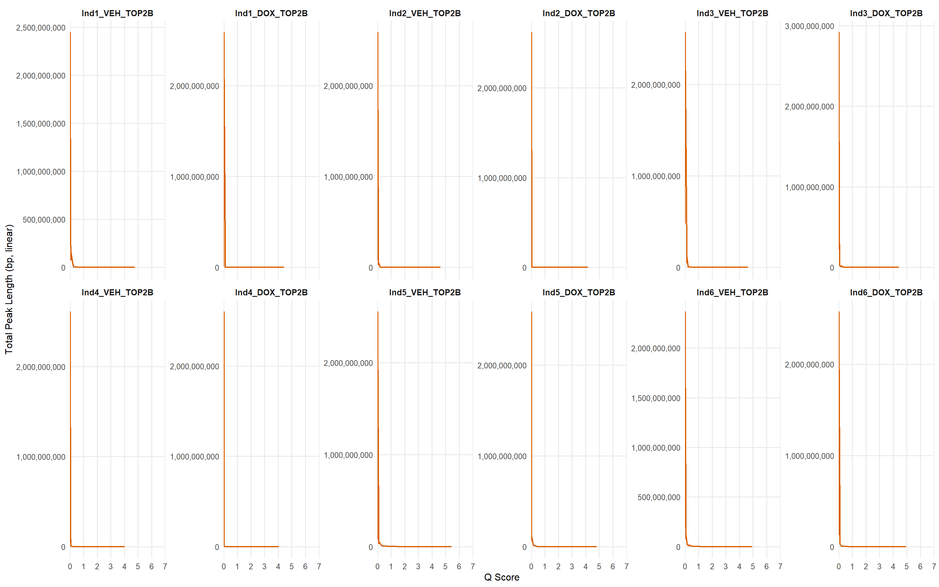
| Version | Author | Date |
|---|---|---|
| bc515e6 | sayanpaul01 | 2025-08-31 |
p_log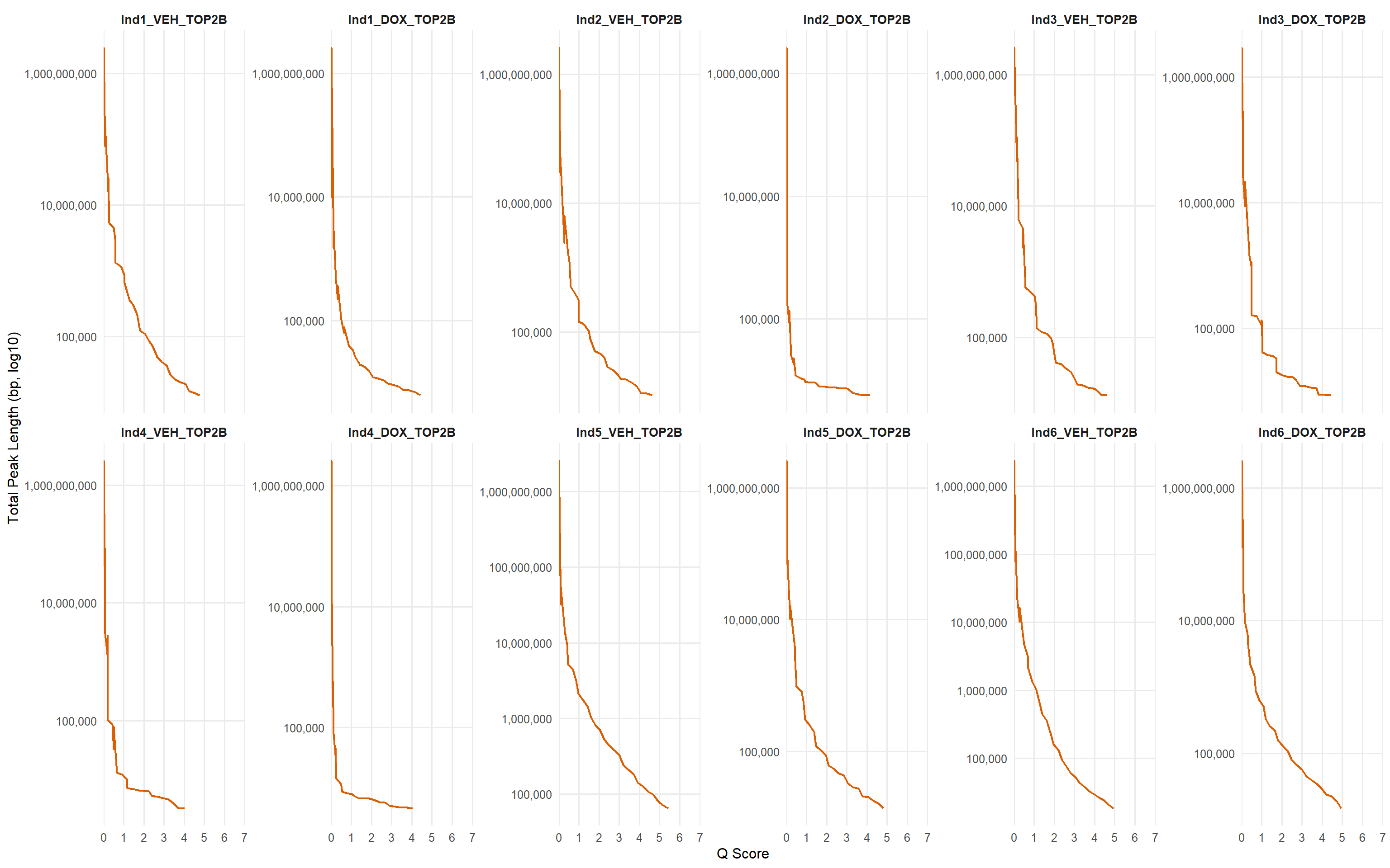
| Version | Author | Date |
|---|---|---|
| bc515e6 | sayanpaul01 | 2025-08-31 |
📌 TOP2B narrow peaks length (before deduplication)
library(tidyverse)
library(readr)
library(scales)

# --- metadata ---
metadata <- tribble(
  ~Sample,           ~Sample_Det,
  "MCW_SP_ChIP27",   "Ind1_VEH_TOP2B",
  "MCW_SP_ChIP28",   "Ind1_DOX_TOP2B",
  "MCW_SP_ChIP31",   "Ind2_VEH_TOP2B",
  "MCW_SP_ChIP32",   "Ind2_DOX_TOP2B",
  "MCW_SP_ChIP39",   "Ind3_VEH_TOP2B",
  "MCW_SP_ChIP40",   "Ind3_DOX_TOP2B",
  "MCW_SP_ChIP43",   "Ind4_VEH_TOP2B",
  "MCW_SP_ChIP44",   "Ind4_DOX_TOP2B",
  "MCW_SP_ChIP51",   "Ind5_VEH_TOP2B",
  "MCW_SP_ChIP52",   "Ind5_DOX_TOP2B",
  "MCW_SP_ChIP55",   "Ind6_VEH_TOP2B",
  "MCW_SP_ChIP56",   "Ind6_DOX_TOP2B"
)

# --- load all cutoff analysis files ---
files <- list.files("data/macs3_narrow_out_TOP2B", pattern = "_cutoff_analysis\\.txt$", full.names = TRUE)

df <- files %>%
  set_names() %>%
  map_dfr(~ read_delim(.x, delim = "\t", show_col_types = FALSE), .id = "filepath") %>%
  mutate(Sample = basename(filepath) %>% str_remove("_cutoff_analysis\\.txt")) %>%
  left_join(metadata, by = "Sample")

# ---- Plot with linear y-axis ----
p_linear <- df %>%
  ggplot(aes(x = qscore, y = lpeaks, group = Sample)) +
  geom_line(size = 0.8, color = "#d95f02") +
  facet_wrap(~ Sample_Det, scales = "free_y", ncol = 6) +
  scale_x_continuous(
    limits = c(0, 7),
    breaks = 0:7,
    labels = as.character(0:7),
    expand = c(0, 0)
  ) +
  scale_y_continuous(labels = label_number(big.mark = ",")) +
  labs(x = "Q Score", y = "Total Peak Length (bp, linear)") +
  theme_minimal(base_size = 12) +
  theme(
    strip.text = element_text(face = "bold", size = 10),
    panel.grid.minor = element_blank()
  )

# ---- Plot with log10 y-axis ----
p_log <- df %>%
  mutate(lpeaks = ifelse(lpeaks <= 0, NA, lpeaks)) %>%
  ggplot(aes(x = qscore, y = lpeaks, group = Sample)) +
  geom_line(size = 0.8, color = "#d95f02") +
  facet_wrap(~ Sample_Det, scales = "free_y", ncol = 6) +
  scale_x_continuous(
    limits = c(0, 7),
    breaks = 0:7,
    labels = as.character(0:7),
    expand = c(0, 0)
  ) +
  scale_y_log10(labels = label_number(big.mark = ",")) +
  labs(x = "Q Score", y = "Total Peak Length (bp, log10)") +
  theme_minimal(base_size = 12) +
  theme(
    strip.text = element_text(face = "bold", size = 10),
    panel.grid.minor = element_blank()
  )

# ---- Print both ----
p_linear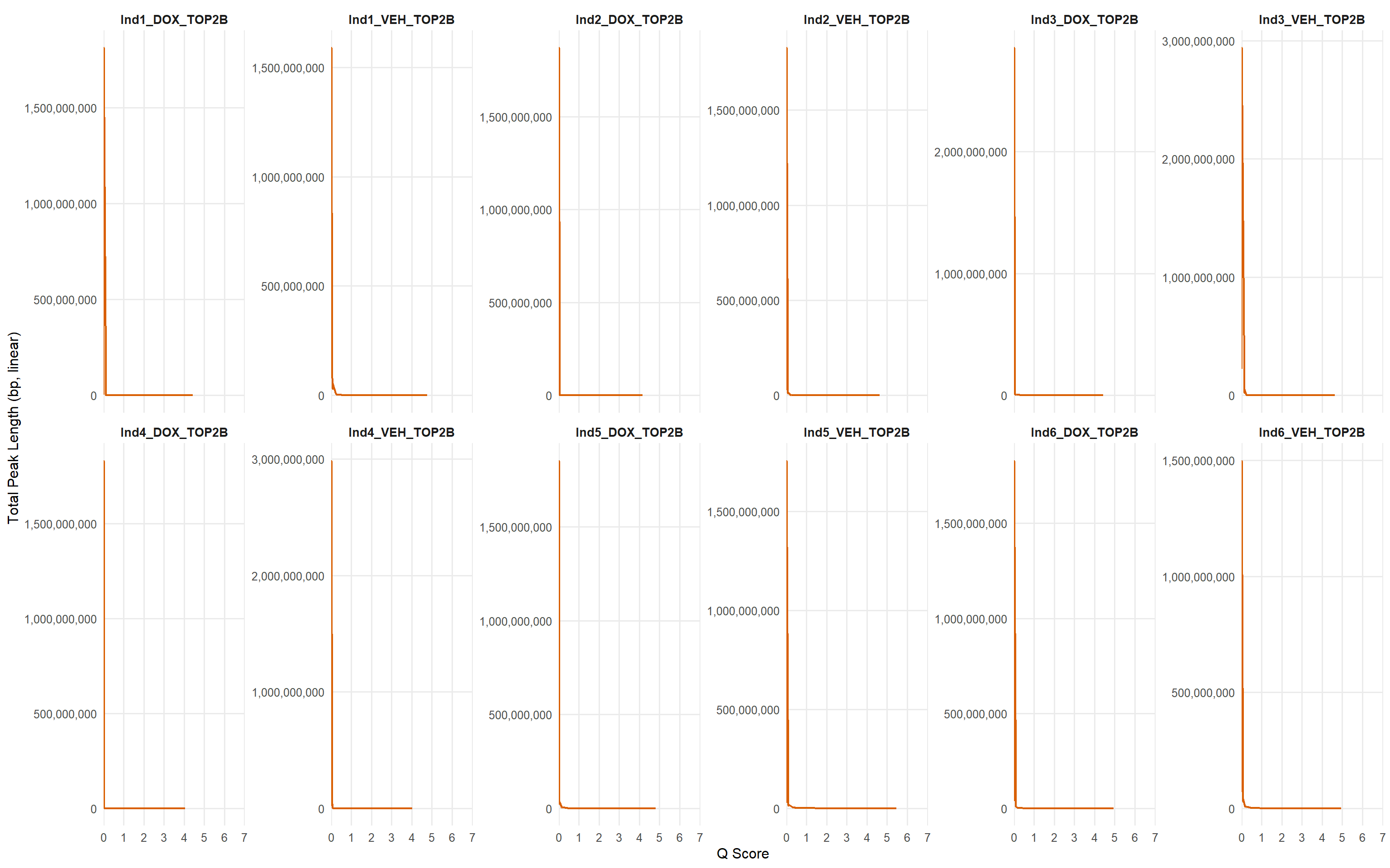
| Version | Author | Date |
|---|---|---|
| bc515e6 | sayanpaul01 | 2025-08-31 |
p_log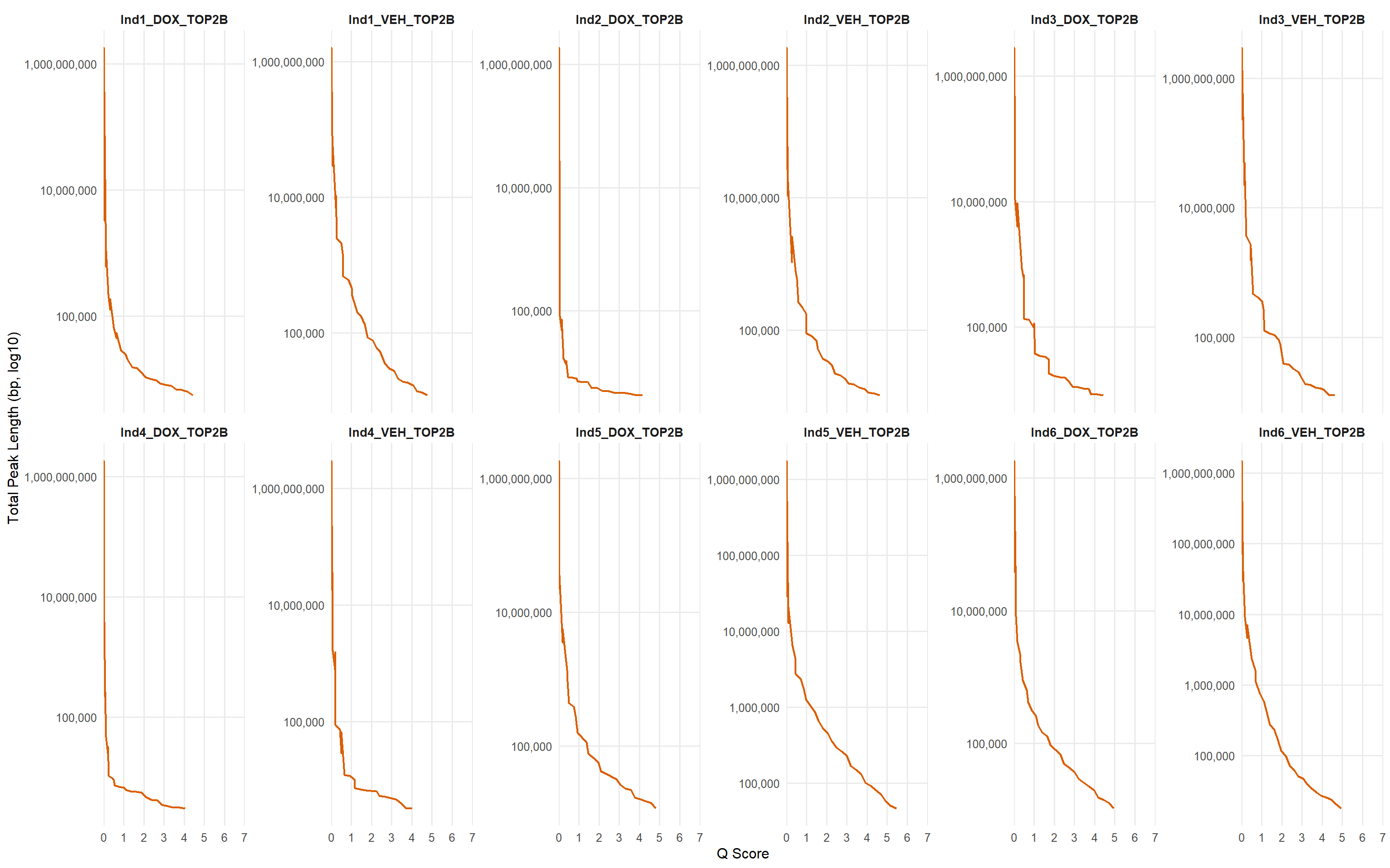
| Version | Author | Date |
|---|---|---|
| bc515e6 | sayanpaul01 | 2025-08-31 |
📌 P53 narrow peaks length (before deduplication)
library(tidyverse)
library(readr)
library(scales)

# --- metadata for p53 ---
metadata_p53 <- tribble(
  ~Sample,           ~Sample_Det,
  "MCW_SP_ChIP29",   "Ind1_VEH_p53",
  "MCW_SP_ChIP30",   "Ind1_DOX_p53",
  "MCW_SP_ChIP33",   "Ind2_VEH_p53",
  "MCW_SP_ChIP34",   "Ind2_DOX_p53",
  "MCW_SP_ChIP41",   "Ind3_VEH_p53",
  "MCW_SP_ChIP42",   "Ind3_DOX_p53",
  "MCW_SP_ChIP45",   "Ind4_VEH_p53",
  "MCW_SP_ChIP46",   "Ind4_DOX_p53",
  "MCW_SP_ChIP53",   "Ind5_VEH_p53",
  "MCW_SP_ChIP54",   "Ind5_DOX_p53",
  "MCW_SP_ChIP57",   "Ind6_VEH_p53",
  "MCW_SP_ChIP58",   "Ind6_DOX_p53"
) %>%
  mutate(
    Sample     = factor(Sample,     levels = Sample),
    Sample_Det = factor(Sample_Det, levels = Sample_Det)
  )

# --- load all cutoff-analysis files ---
data_dir <- "data/macs3_narrow_out_P53"   # adjust if needed
files <- list.files(data_dir, pattern = "_cutoff_analysis\\.txt$", full.names = TRUE)

df_p53 <- files %>%
  set_names() %>%
  map_dfr(~ read_delim(.x, delim = "\t", show_col_types = FALSE), .id = "filepath") %>%
  mutate(Sample = basename(filepath) %>% str_remove("_cutoff_analysis\\.txt")) %>%
  left_join(metadata_p53, by = "Sample") %>%
  mutate(Sample_Det = factor(Sample_Det, levels = levels(metadata_p53$Sample_Det))) %>%
  arrange(Sample_Det, qscore)

# --------- common x scale (forces 0..7 with a printed 0) ----------
x_fixed <- scale_x_continuous(
  limits = c(0, 7),
  breaks = 0:7,
  labels = as.character(0:7),
  expand = c(0, 0)
)

# ---- linear y ----
p_linear_p53 <- ggplot(df_p53, aes(qscore, lpeaks, group = Sample)) +
  geom_line(size = 0.8, color = "#d95f02") +
  facet_wrap(~ Sample_Det, scales = "free_y", ncol = 6) +
  x_fixed +
  scale_y_continuous(labels = label_number(big.mark = ",")) +
  labs(x = "Q Score", y = "Total Peak Length (bp, linear)") +
  theme_minimal(base_size = 12) +
  theme(
    strip.text = element_text(face = "bold", size = 10),
    panel.grid.minor = element_blank()
  )

# ---- log10 y ----
p_log_p53 <- df_p53 %>%
  mutate(lpeaks = ifelse(lpeaks <= 0, NA, lpeaks)) %>%
  ggplot(aes(qscore, lpeaks, group = Sample)) +
  geom_line(size = 0.8, color = "#d95f02") +
  facet_wrap(~ Sample_Det, scales = "free_y", ncol = 6) +
  x_fixed +
  scale_y_log10(labels = label_number(big.mark = ",")) +
  labs(x = "Q Score", y = "Total Peak Length (bp, log10)") +
  theme_minimal(base_size = 12) +
  theme(
    strip.text = element_text(face = "bold", size = 10),
    panel.grid.minor = element_blank()
  )

# ---- show both ----
p_linear_p53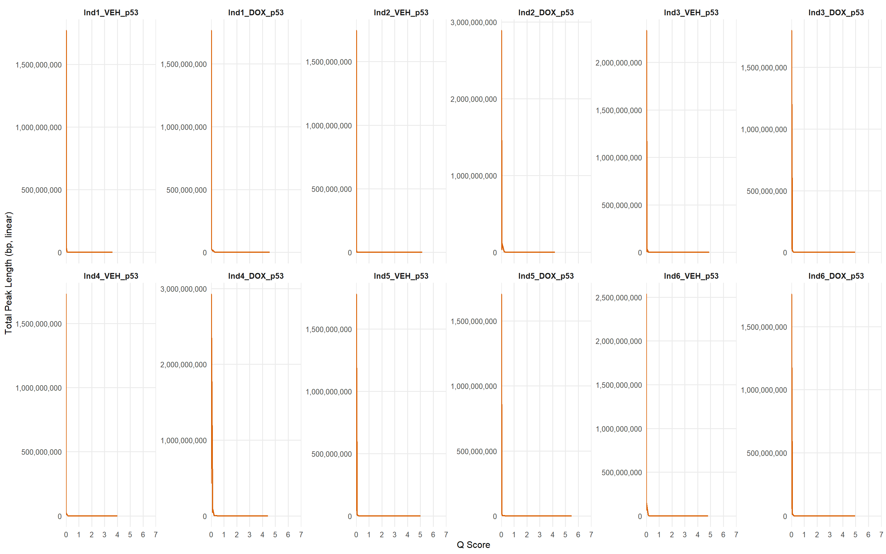
| Version | Author | Date |
|---|---|---|
| bc515e6 | sayanpaul01 | 2025-08-31 |
p_log_p53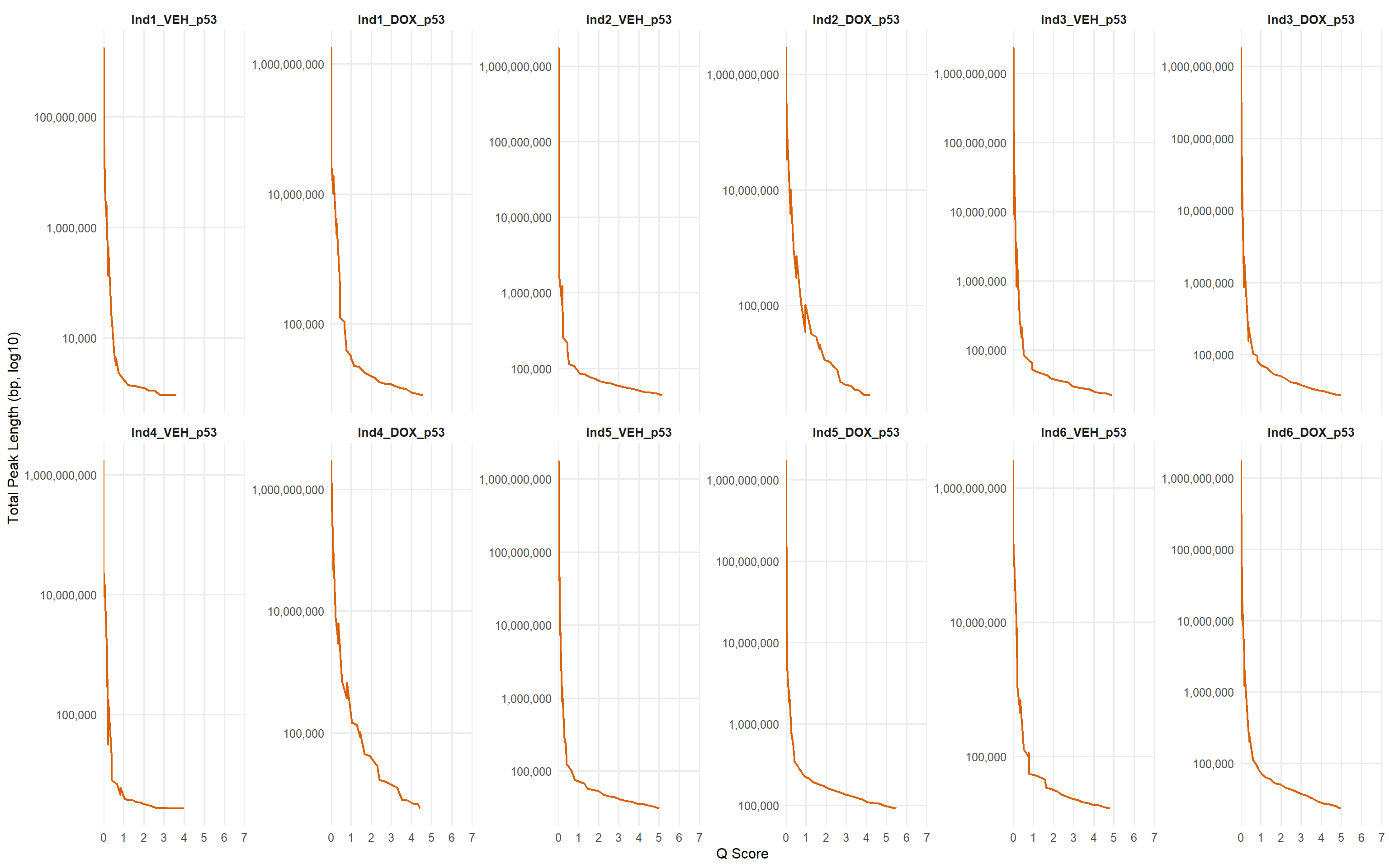
| Version | Author | Date |
|---|---|---|
| bc515e6 | sayanpaul01 | 2025-08-31 |
📌 TOP2B broad peaks length (after deduplication)
library(tidyverse)
library(readr)
library(scales)

# --- metadata ---
metadata <- tribble(
  ~Sample,           ~Sample_Det,
  "MCW_SP_ChIP27",   "Ind1_VEH_TOP2B",
  "MCW_SP_ChIP28",   "Ind1_DOX_TOP2B",
  "MCW_SP_ChIP31",   "Ind2_VEH_TOP2B",
  "MCW_SP_ChIP32",   "Ind2_DOX_TOP2B",
  "MCW_SP_ChIP39",   "Ind3_VEH_TOP2B",
  "MCW_SP_ChIP40",   "Ind3_DOX_TOP2B",
  "MCW_SP_ChIP43",   "Ind4_VEH_TOP2B",
  "MCW_SP_ChIP44",   "Ind4_DOX_TOP2B",
  "MCW_SP_ChIP51",   "Ind5_VEH_TOP2B",
  "MCW_SP_ChIP52",   "Ind5_DOX_TOP2B",
  "MCW_SP_ChIP55",   "Ind6_VEH_TOP2B",
  "MCW_SP_ChIP56",   "Ind6_DOX_TOP2B"
)

# --- load all cutoff analysis files ---
files <- list.files("data/macs3_broad_out_TOP2B_dedup", pattern = "_cutoff_analysis\\.txt$", full.names = TRUE)

df <- files %>%
  set_names() %>%
  map_dfr(~ read_delim(.x, delim = "\t", show_col_types = FALSE), .id = "filepath") %>%
  mutate(Sample = basename(filepath) %>% str_remove("_cutoff_analysis\\.txt")) %>%
  left_join(metadata, by = "Sample")

# ---- Plot with linear y-axis ----
p_linear <- df %>%
  ggplot(aes(x = qscore, y = lpeaks, group = Sample)) +
  geom_line(size = 0.8, color = "#d95f02") +
  facet_wrap(~ Sample_Det, scales = "free_y", ncol = 6) +
  scale_x_continuous(
    limits = c(0, 7),
    breaks = 0:7,
    labels = as.character(0:7),
    expand = c(0, 0)
  ) +
  scale_y_continuous(labels = label_number(big.mark = ",")) +
  labs(x = "Q Score", y = "Total Peak Length (bp, linear)") +
  theme_minimal(base_size = 12) +
  theme(
    strip.text = element_text(face = "bold", size = 10),
    panel.grid.minor = element_blank()
  )

# ---- Plot with log10 y-axis ----
p_log <- df %>%
  mutate(lpeaks = ifelse(lpeaks <= 0, NA, lpeaks)) %>%
  ggplot(aes(x = qscore, y = lpeaks, group = Sample)) +
  geom_line(size = 0.8, color = "#d95f02") +
  facet_wrap(~ Sample_Det, scales = "free_y", ncol = 6) +
  scale_x_continuous(
    limits = c(0, 7),
    breaks = 0:7,
    labels = as.character(0:7),
    expand = c(0, 0)
  ) +
  scale_y_log10(labels = label_number(big.mark = ",")) +
  labs(x = "Q Score", y = "Total Peak Length (bp, log10)") +
  theme_minimal(base_size = 12) +
  theme(
    strip.text = element_text(face = "bold", size = 10),
    panel.grid.minor = element_blank()
  )

# ---- Print both ----
p_linear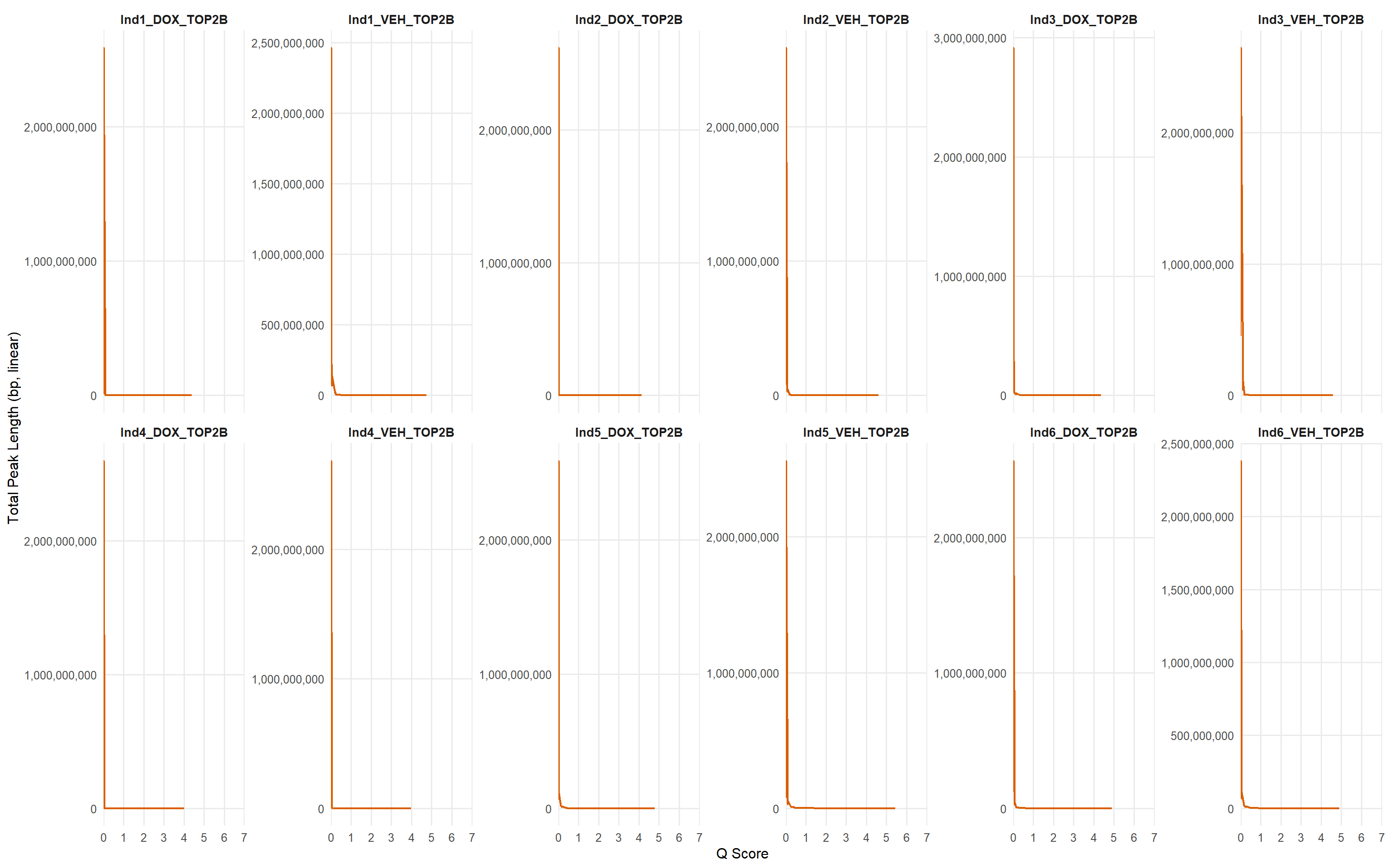
| Version | Author | Date |
|---|---|---|
| bc515e6 | sayanpaul01 | 2025-08-31 |
p_log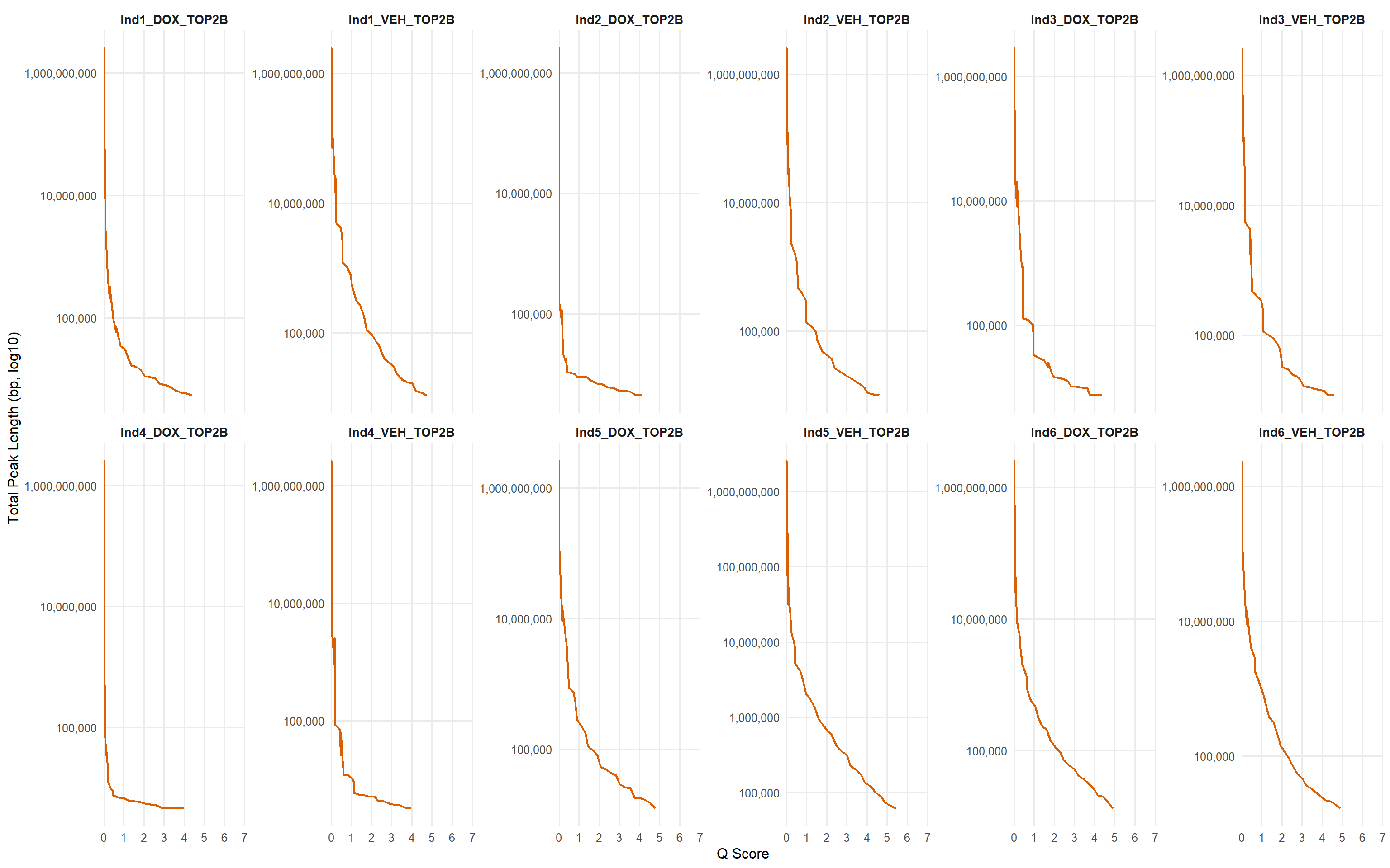
| Version | Author | Date |
|---|---|---|
| bc515e6 | sayanpaul01 | 2025-08-31 |
📌 TOP2B narrow peaks length (after deduplication)
library(tidyverse)
library(readr)
library(scales)

# --- metadata ---
metadata <- tribble(
  ~Sample,           ~Sample_Det,
  "MCW_SP_ChIP27",   "Ind1_VEH_TOP2B",
  "MCW_SP_ChIP28",   "Ind1_DOX_TOP2B",
  "MCW_SP_ChIP31",   "Ind2_VEH_TOP2B",
  "MCW_SP_ChIP32",   "Ind2_DOX_TOP2B",
  "MCW_SP_ChIP39",   "Ind3_VEH_TOP2B",
  "MCW_SP_ChIP40",   "Ind3_DOX_TOP2B",
  "MCW_SP_ChIP43",   "Ind4_VEH_TOP2B",
  "MCW_SP_ChIP44",   "Ind4_DOX_TOP2B",
  "MCW_SP_ChIP51",   "Ind5_VEH_TOP2B",
  "MCW_SP_ChIP52",   "Ind5_DOX_TOP2B",
  "MCW_SP_ChIP55",   "Ind6_VEH_TOP2B",
  "MCW_SP_ChIP56",   "Ind6_DOX_TOP2B"
)

# --- load all cutoff analysis files ---
files <- list.files("data/macs3_narrow_out_TOP2B_dedup", pattern = "_cutoff_analysis\\.txt$", full.names = TRUE)

df <- files %>%
  set_names() %>%
  map_dfr(~ read_delim(.x, delim = "\t", show_col_types = FALSE), .id = "filepath") %>%
  mutate(Sample = basename(filepath) %>% str_remove("_cutoff_analysis\\.txt")) %>%
  left_join(metadata, by = "Sample")

# ---- Plot with linear y-axis ----
p_linear <- df %>%
  ggplot(aes(x = qscore, y = lpeaks, group = Sample)) +
  geom_line(size = 0.8, color = "#d95f02") +
  facet_wrap(~ Sample_Det, scales = "free_y", ncol = 6) +
  scale_x_continuous(
    limits = c(0, 7),
    breaks = 0:7,
    labels = as.character(0:7),
    expand = c(0, 0)
  ) +
  scale_y_continuous(labels = label_number(big.mark = ",")) +
  labs(x = "Q Score", y = "Total Peak Length (bp, linear)") +
  theme_minimal(base_size = 12) +
  theme(
    strip.text = element_text(face = "bold", size = 10),
    panel.grid.minor = element_blank()
  )

# ---- Plot with log10 y-axis ----
p_log <- df %>%
  mutate(lpeaks = ifelse(lpeaks <= 0, NA, lpeaks)) %>%
  ggplot(aes(x = qscore, y = lpeaks, group = Sample)) +
  geom_line(size = 0.8, color = "#d95f02") +
  facet_wrap(~ Sample_Det, scales = "free_y", ncol = 6) +
  scale_x_continuous(
    limits = c(0, 7),
    breaks = 0:7,
    labels = as.character(0:7),
    expand = c(0, 0)
  ) +
  scale_y_log10(labels = label_number(big.mark = ",")) +
  labs(x = "Q Score", y = "Total Peak Length (bp, log10)") +
  theme_minimal(base_size = 12) +
  theme(
    strip.text = element_text(face = "bold", size = 10),
    panel.grid.minor = element_blank()
  )

# ---- Print both ----
p_linear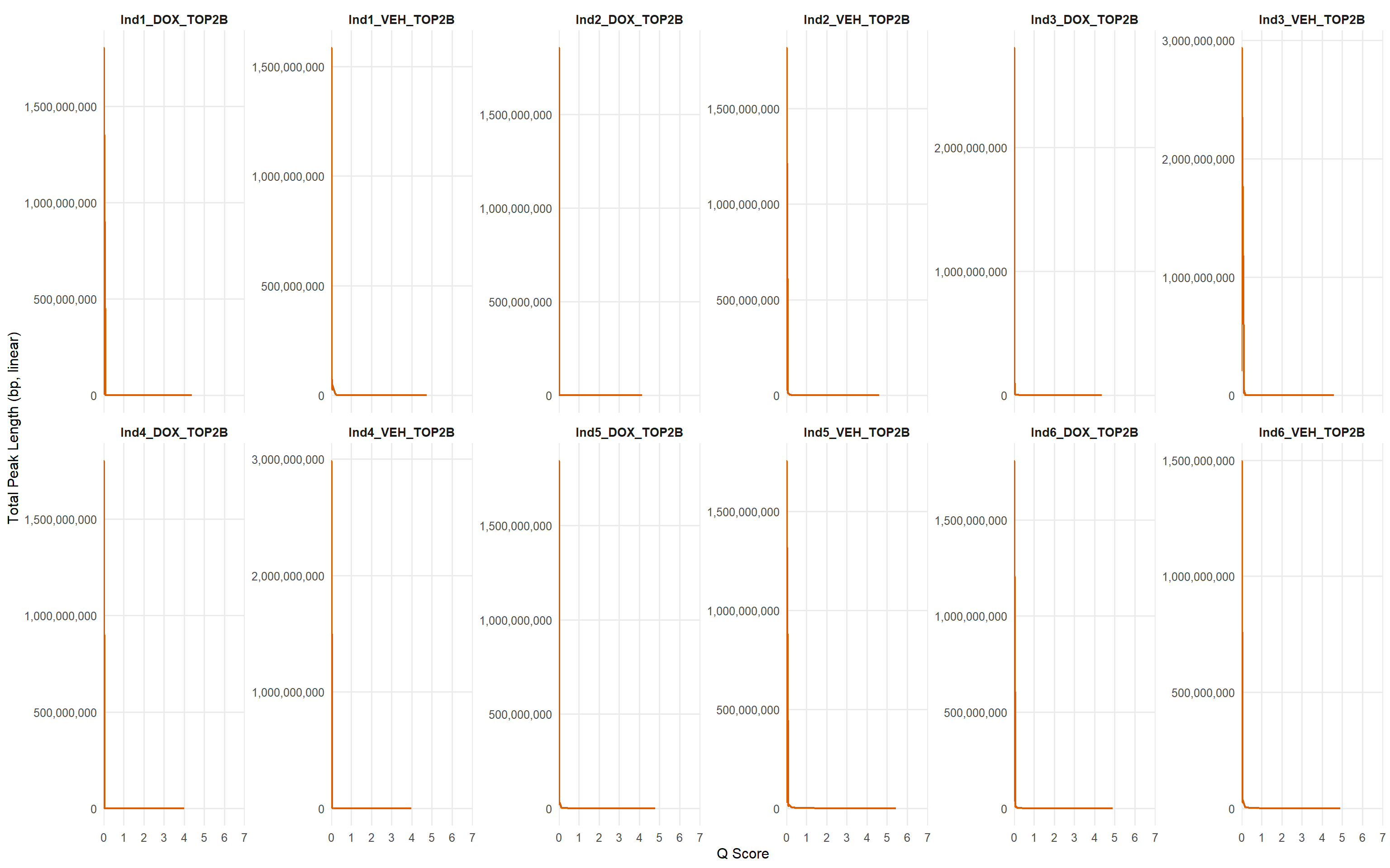
| Version | Author | Date |
|---|---|---|
| bc515e6 | sayanpaul01 | 2025-08-31 |
p_log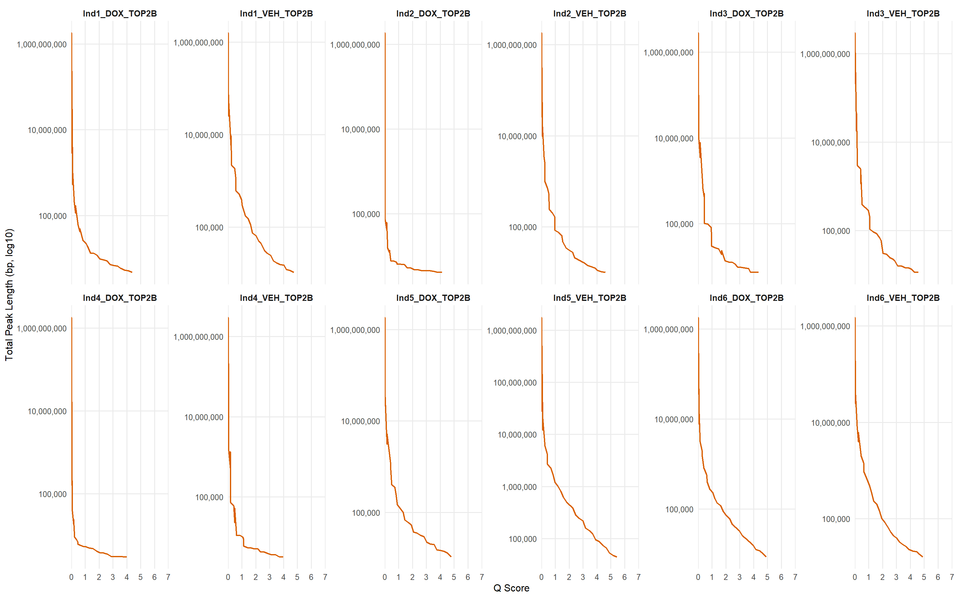
| Version | Author | Date |
|---|---|---|
| bc515e6 | sayanpaul01 | 2025-08-31 |
📌 P53 narrow peaks length (after deduplication)
library(tidyverse)
library(readr)
library(scales)

# --- metadata for p53 ---
metadata_p53 <- tribble(
  ~Sample,           ~Sample_Det,
  "MCW_SP_ChIP29",   "Ind1_VEH_p53",
  "MCW_SP_ChIP30",   "Ind1_DOX_p53",
  "MCW_SP_ChIP33",   "Ind2_VEH_p53",
  "MCW_SP_ChIP34",   "Ind2_DOX_p53",
  "MCW_SP_ChIP41",   "Ind3_VEH_p53",
  "MCW_SP_ChIP42",   "Ind3_DOX_p53",
  "MCW_SP_ChIP45",   "Ind4_VEH_p53",
  "MCW_SP_ChIP46",   "Ind4_DOX_p53",
  "MCW_SP_ChIP53",   "Ind5_VEH_p53",
  "MCW_SP_ChIP54",   "Ind5_DOX_p53",
  "MCW_SP_ChIP57",   "Ind6_VEH_p53",
  "MCW_SP_ChIP58",   "Ind6_DOX_p53"
) %>%
  mutate(
    Sample     = factor(Sample,     levels = Sample),
    Sample_Det = factor(Sample_Det, levels = Sample_Det)
  )

# --- load all cutoff-analysis files ---
data_dir <- "data/macs3_narrow_out_P53_dedup"
files <- list.files(data_dir, pattern = "_cutoff_analysis\\.txt$", full.names = TRUE)

df_p53 <- files %>%
  set_names() %>%
  map_dfr(~ read_delim(.x, delim = "\t", show_col_types = FALSE), .id = "filepath") %>%
  mutate(Sample = basename(filepath) %>% str_remove("_cutoff_analysis\\.txt")) %>%
  left_join(metadata_p53, by = "Sample") %>%
  mutate(Sample_Det = factor(Sample_Det, levels = levels(metadata_p53$Sample_Det))) %>%
  arrange(Sample_Det, qscore)

# --------- common x scale (forces 0..7 with a printed 0) ----------
x_fixed <- scale_x_continuous(
  limits = c(0, 7),
  breaks = 0:7,
  labels = as.character(0:7),
  expand = c(0, 0)
)

# ---- linear y (lpeaks) ----
p_linear_p53 <- ggplot(df_p53, aes(qscore, lpeaks, group = Sample)) +
  geom_line(size = 0.8, color = "#d95f02") +
  facet_wrap(~ Sample_Det, scales = "free_y", ncol = 6) +
  x_fixed +
  scale_y_continuous(labels = label_number(big.mark = ",")) +
  labs(x = "Q Score", y = "Total Peak Length (bp, linear)") +
  theme_minimal(base_size = 12) +
  theme(
    strip.text = element_text(face = "bold", size = 10),
    panel.grid.minor = element_blank()
  )

# ---- log10 y (lpeaks) ----
p_log_p53 <- df_p53 %>%
  mutate(lpeaks = ifelse(lpeaks <= 0, NA, lpeaks)) %>%
  ggplot(aes(qscore, lpeaks, group = Sample)) +
  geom_line(size = 0.8, color = "#d95f02") +
  facet_wrap(~ Sample_Det, scales = "free_y", ncol = 6) +
  x_fixed +
  scale_y_log10(labels = label_number(big.mark = ",")) +
  labs(x = "Q Score", y = "Total Peak Length (bp, log10)") +
  theme_minimal(base_size = 12) +
  theme(
    strip.text = element_text(face = "bold", size = 10),
    panel.grid.minor = element_blank()
  )

# ---- show both ----
p_linear_p53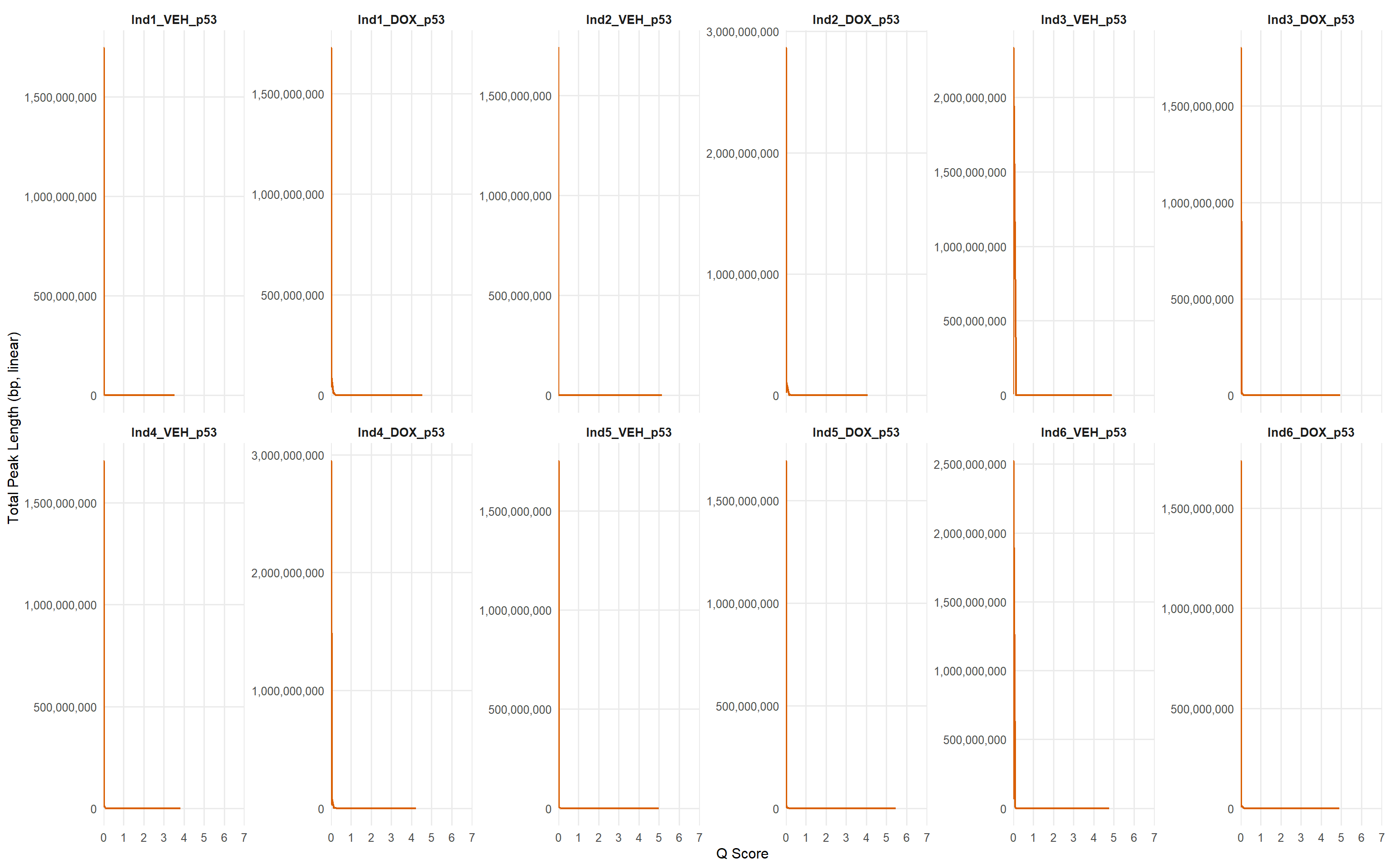
| Version | Author | Date |
|---|---|---|
| bc515e6 | sayanpaul01 | 2025-08-31 |
p_log_p53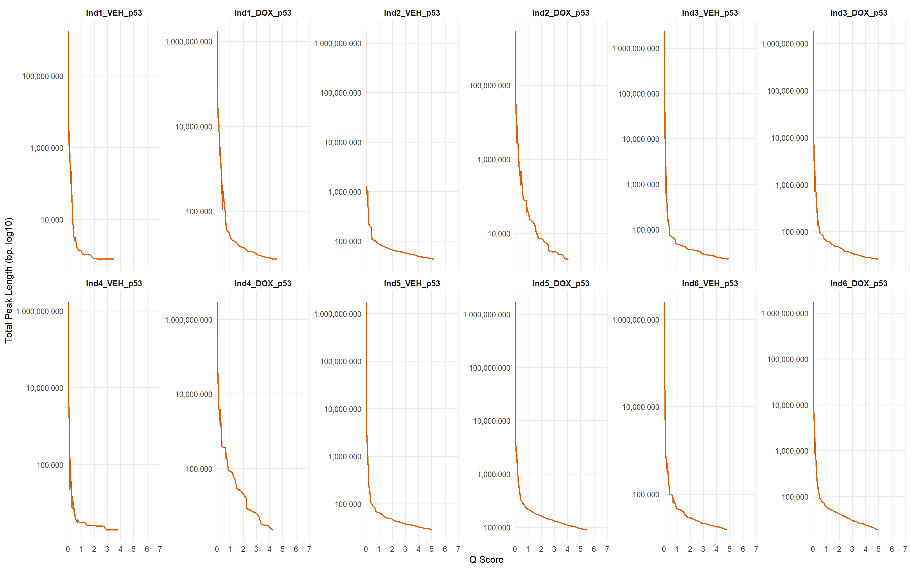
| Version | Author | Date |
|---|---|---|
| bc515e6 | sayanpaul01 | 2025-08-31 |
📌 Elbow cutoff TOP2B broad peaks (before deduplication)
suppressPackageStartupMessages({
  library(tidyverse)
  library(readr)
  library(scales)
  library(stringr)
})

# ---- Load data ----
df <- read_csv("data/ELBOW_TOP2B_broad.csv", show_col_types = FALSE)

# ---- Ensure numeric + derive Individual ID and ordered Tx ----
num_cols <- c("Elbow_cutoff_Qscore", "NPeaks_at_cutoff", "LPeaks_at_cutoff")
df <- df %>% mutate(across(all_of(num_cols), as.numeric))

# Robust 'Ind' derivation
if ("Ind_ab" %in% names(df)) {
  df <- df %>% mutate(Ind = str_extract(Ind_ab, "^Ind\\d+"))
} else if ("Sample Det" %in% names(df)) {
  df <- df %>% mutate(Ind = str_extract(`Sample Det`, "^Ind\\d+"))
} else {
  df <- df %>% mutate(Ind = Sample)
}

# Order Tx: VEH → DOX
df <- df %>% mutate(Tx = factor(Tx, levels = c("VEH", "DOX")))

# ---- Long format for plotting ----
df_long <- df %>%
  select(Sample, Ind, Tx, Elbow_cutoff_Qscore, NPeaks_at_cutoff, LPeaks_at_cutoff) %>%
  pivot_longer(
    cols = c(NPeaks_at_cutoff, LPeaks_at_cutoff, Elbow_cutoff_Qscore),
    names_to = "metric", values_to = "value"
  ) %>%
  mutate(metric = recode(
    metric,
    NPeaks_at_cutoff     = "NPeaks at elbow",
    LPeaks_at_cutoff     = "LPeaks at elbow (bp)",
    Elbow_cutoff_Qscore  = "Elbow cutoff (−log10 q)"
  ))

# ---- Color palette (Okabe–Ito for up to 8 individuals) ----
okabe_ito <- c(
  "#E69F00", "#56B4E9", "#009E73",
  "#F0E442", "#0072B2", "#D55E00",
  "#CC79A7", "#999999"
)
n_ind <- df %>% distinct(Ind) %>% nrow()

col_scale <- if (n_ind <= length(okabe_ito)) {
  scale_color_manual(values = okabe_ito)
} else {
  scale_color_viridis_d(option = "C", end = 0.95)
}

# ---- Plot: Paired slopes VEH → DOX per individual ----
p_slope <- ggplot(df_long, aes(x = Tx, y = value, group = Ind, color = Ind)) +
  geom_line(linewidth = 1.2, alpha = 0.9) +
  geom_point(size = 3) +
  facet_wrap(~ metric, scales = "free_y", ncol = 3) +
  scale_y_continuous(labels = label_number(big.mark = ",")) +
  col_scale +
  labs(
    title = "Elbow cutoff TOP2B broad peaks (before dedup)",
    x = NULL, y = NULL, color = "Individual"
  ) +
  theme_minimal(base_size = 13) +
  theme(
    legend.position = "bottom",
    legend.text = element_text(size = 10),
    strip.text = element_text(face = "bold")
  )

# ---- Show plot ----
print(p_slope)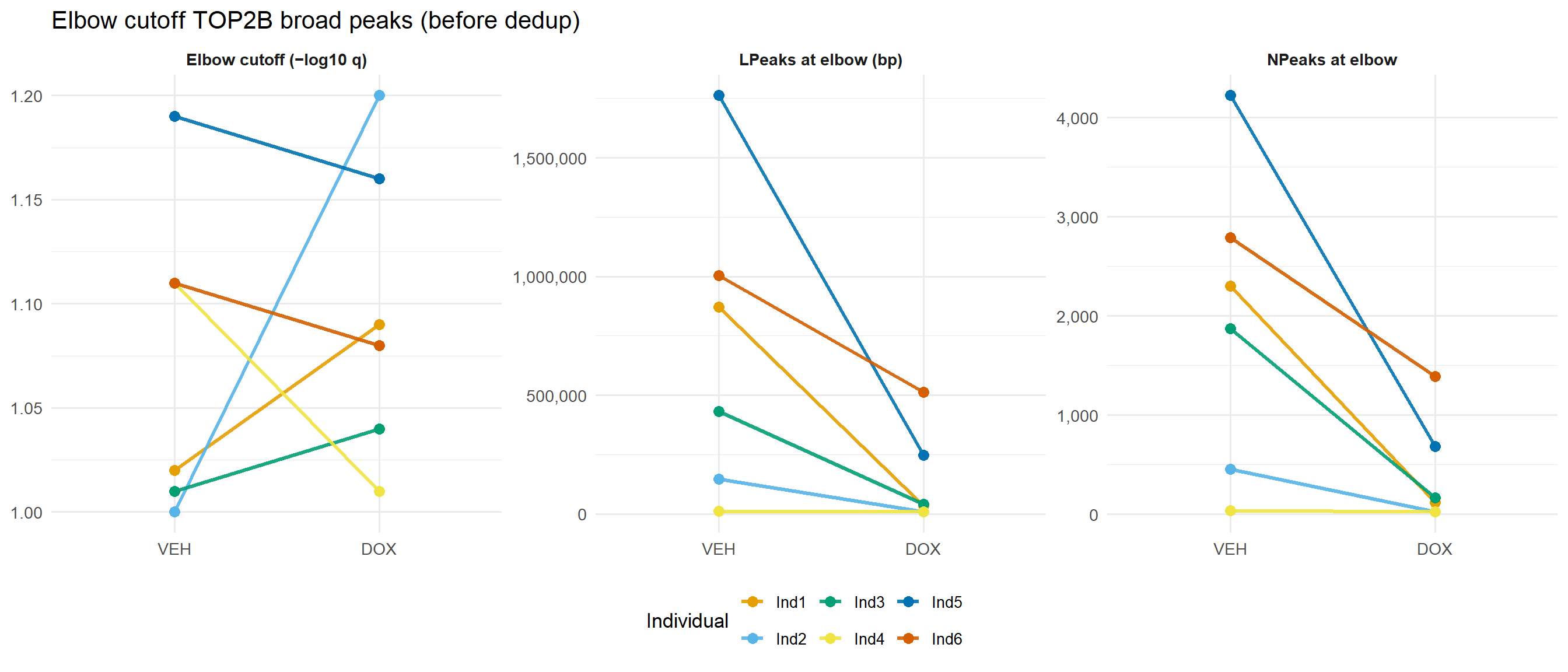
📌 Elbow cutoff TOP2B narrow peaks (before deduplication)
suppressPackageStartupMessages({
  library(tidyverse)
  library(readr)
  library(scales)
  library(stringr)
})

# ---- Load data ----
df <- read_csv("data/ELBOW_TOP2B_narrow.csv", show_col_types = FALSE)

# ---- Harmonize column names (supports both naming schemes) ----
if ("Elbow_qscore" %in% names(df)) df <- df %>% rename(Elbow_cutoff_Qscore = Elbow_qscore)
if ("NPeaks_at_elbow" %in% names(df)) df <- df %>% rename(NPeaks_at_cutoff = NPeaks_at_elbow)
if ("LPeaks_at_elbow" %in% names(df)) df <- df %>% rename(LPeaks_at_cutoff = LPeaks_at_elbow)

# ---- Ensure numeric + derive Individual ID and ordered Tx ----
num_cols <- c("Elbow_cutoff_Qscore", "NPeaks_at_cutoff", "LPeaks_at_cutoff")
df <- df %>% mutate(across(all_of(num_cols), as.numeric))

# Robust 'Ind' derivation
if ("Ind_ab" %in% names(df)) {
  df <- df %>% mutate(Ind = str_extract(Ind_ab, "^Ind\\d+"))
} else if ("Sample Det" %in% names(df)) {
  df <- df %>% mutate(Ind = str_extract(`Sample Det`, "^Ind\\d+"))
} else {
  df <- df %>% mutate(Ind = Sample)
}

# Order Tx: VEH → DOX (handle both Tx or Treatment columns)
if ("Tx" %in% names(df)) {
  df <- df %>% mutate(Tx = factor(Tx, levels = c("VEH","DOX")))
} else if ("Treatment" %in% names(df)) {
  df <- df %>% mutate(Tx = factor(Treatment, levels = c("VEH_TOP2B","DOX_TOP2B")))
}

# ---- Long format for plotting ----
df_long <- df %>%
  select(Sample, Ind, Tx, Elbow_cutoff_Qscore, NPeaks_at_cutoff, LPeaks_at_cutoff) %>%
  pivot_longer(
    cols = c(NPeaks_at_cutoff, LPeaks_at_cutoff, Elbow_cutoff_Qscore),
    names_to = "metric", values_to = "value"
  ) %>%
  mutate(metric = recode(
    metric,
    NPeaks_at_cutoff     = "NPeaks at elbow",
    LPeaks_at_cutoff     = "LPeaks at elbow (bp)",
    Elbow_cutoff_Qscore  = "Elbow cutoff (−log10 q)"
  ))

# ---- Color palette (Okabe–Ito up to 8 individuals, else viridis) ----
okabe_ito <- c("#E69F00","#56B4E9","#009E73","#F0E442","#0072B2","#D55E00","#CC79A7","#999999")
n_ind <- df %>% distinct(Ind) %>% nrow()
col_scale <- if (n_ind <= length(okabe_ito)) {
  scale_color_manual(values = okabe_ito)
} else {
  scale_color_viridis_d(option = "C", end = 0.95)
}

# ---- Plot: Paired slopes VEH → DOX per individual ----
p_slope <- ggplot(df_long, aes(x = Tx, y = value, group = Ind, color = Ind)) +
  geom_line(linewidth = 1.2, alpha = 0.9) +
  geom_point(size = 3) +
  facet_wrap(~ metric, scales = "free_y", ncol = 3) +
  scale_y_continuous(labels = label_number(big.mark = ",")) +
  col_scale +
  labs(
    title = "Elbow cutoff TOP2B narrow peaks (before dedup)",
    x = NULL, y = NULL, color = "Individual"
  ) +
  theme_minimal(base_size = 13) +
  theme(
    legend.position = "bottom",
    legend.text = element_text(size = 10),
    strip.text = element_text(face = "bold")
  )

print(p_slope)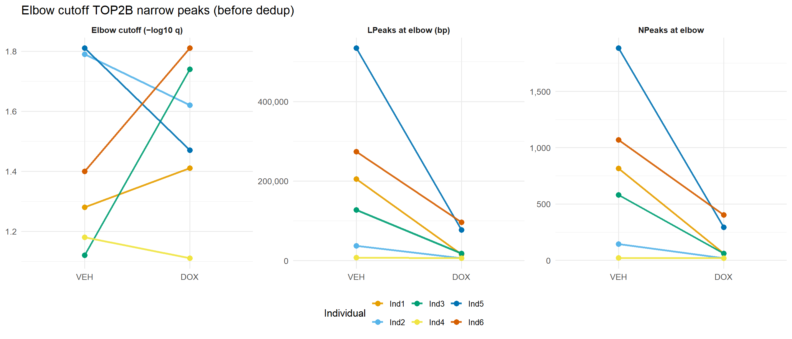
sessionInfo()R version 4.3.0 (2023-04-21 ucrt)
Platform: x86_64-w64-mingw32/x64 (64-bit)
Running under: Windows 11 x64 (build 26100)
Matrix products: default
locale:
[1] LC_COLLATE=English_United States.utf8
[2] LC_CTYPE=English_United States.utf8
[3] LC_MONETARY=English_United States.utf8
[4] LC_NUMERIC=C
[5] LC_TIME=English_United States.utf8
time zone: America/Chicago
tzcode source: internal
attached base packages:
[1] stats graphics grDevices utils datasets methods base
other attached packages:
[1] scales_1.3.0 lubridate_1.9.4 forcats_1.0.0 stringr_1.5.1
[5] dplyr_1.1.4 purrr_1.0.4 readr_2.1.5 tidyr_1.3.1
[9] tibble_3.2.1 ggplot2_3.5.2 tidyverse_2.0.0
loaded via a namespace (and not attached):
[1] sass_0.4.10 generics_0.1.3 stringi_1.8.3 hms_1.1.3
[5] digest_0.6.34 magrittr_2.0.3 evaluate_1.0.3 grid_4.3.0
[9] timechange_0.3.0 fastmap_1.2.0 rprojroot_2.0.4 workflowr_1.7.1
[13] jsonlite_2.0.0 whisker_0.4.1 promises_1.3.2 jquerylib_0.1.4
[17] cli_3.6.1 crayon_1.5.3 rlang_1.1.3 bit64_4.6.0-1
[21] munsell_0.5.1 withr_3.0.2 cachem_1.1.0 yaml_2.3.10
[25] parallel_4.3.0 tools_4.3.0 tzdb_0.5.0 colorspace_2.1-0
[29] httpuv_1.6.15 vctrs_0.6.5 R6_2.6.1 lifecycle_1.0.4
[33] git2r_0.36.2 bit_4.6.0 fs_1.6.3 vroom_1.6.5
[37] pkgconfig_2.0.3 pillar_1.10.2 bslib_0.9.0 later_1.3.2
[41] gtable_0.3.6 glue_1.7.0 Rcpp_1.0.12 xfun_0.52
[45] tidyselect_1.2.1 rstudioapi_0.17.1 knitr_1.50 farver_2.1.2
[49] htmltools_0.5.8.1 labeling_0.4.3 rmarkdown_2.29 compiler_4.3.0