Function and Pathway Enrichment Analysis
Last updated: 2025-06-04
Checks: 6 1
Knit directory: CX5461_Project/
This reproducible R Markdown analysis was created with workflowr (version 1.7.1). The Checks tab describes the reproducibility checks that were applied when the results were created. The Past versions tab lists the development history.
The R Markdown file has unstaged changes. To know which version of
the R Markdown file created these results, you’ll want to first commit
it to the Git repo. If you’re still working on the analysis, you can
ignore this warning. When you’re finished, you can run
wflow_publish to commit the R Markdown file and build the
HTML.
Great job! The global environment was empty. Objects defined in the global environment can affect the analysis in your R Markdown file in unknown ways. For reproduciblity it’s best to always run the code in an empty environment.
The command set.seed(20250129) was run prior to running
the code in the R Markdown file. Setting a seed ensures that any results
that rely on randomness, e.g. subsampling or permutations, are
reproducible.
Great job! Recording the operating system, R version, and package versions is critical for reproducibility.
Nice! There were no cached chunks for this analysis, so you can be confident that you successfully produced the results during this run.
Great job! Using relative paths to the files within your workflowr project makes it easier to run your code on other machines.
Great! You are using Git for version control. Tracking code development and connecting the code version to the results is critical for reproducibility.
The results in this page were generated with repository version 75100b0. See the Past versions tab to see a history of the changes made to the R Markdown and HTML files.
Note that you need to be careful to ensure that all relevant files for
the analysis have been committed to Git prior to generating the results
(you can use wflow_publish or
wflow_git_commit). workflowr only checks the R Markdown
file, but you know if there are other scripts or data files that it
depends on. Below is the status of the Git repository when the results
were generated:
Ignored files:
    Ignored:    .RData
    Ignored:    .Rhistory
    Ignored:    .Rproj.user/
    Ignored:    0.1 box.svg
    Ignored:    Rplot04.svg
    Ignored:    analysis/Corrmotif_Conc.html
    Ignored:    analysis/figure/

Untracked files:
    Untracked:  0.1 density.svg
    Untracked:  0.1.emf
    Untracked:  0.1.svg
    Untracked:  0.5 box.svg
    Untracked:  0.5 density.svg
    Untracked:  0.5.svg
    Untracked:  Additional/
    Untracked:  Autosome factors.svg
    Untracked:  CX_5461_Pattern_Genes_24hr.csv
    Untracked:  CX_5461_Pattern_Genes_3hr.csv
    Untracked:  Cell viability box plot.svg
    Untracked:  DEG GO terms.svg
    Untracked:  DNA damage associated GO terms.svg
    Untracked:  DRC1.svg
    Untracked:  Figure 1.jpeg
    Untracked:  Figure 1.pdf
    Untracked:  Figure_CM_Purity.pdf
    Untracked:  G Quadruplex DEGs.svg
    Untracked:  PC2 Vs PC3 Autosome.svg
    Untracked:  PCA autosome.svg
    Untracked:  Rplot 18.svg
    Untracked:  Rplot.svg
    Untracked:  Rplot01.svg
    Untracked:  Rplot02.svg
    Untracked:  Rplot03.svg
    Untracked:  Rplot05.svg
    Untracked:  Rplot06.svg
    Untracked:  Rplot07.svg
    Untracked:  Rplot08.jpeg
    Untracked:  Rplot08.svg
    Untracked:  Rplot09.svg
    Untracked:  Rplot10.svg
    Untracked:  Rplot11.svg
    Untracked:  Rplot12.svg
    Untracked:  Rplot13.svg
    Untracked:  Rplot14.svg
    Untracked:  Rplot15.svg
    Untracked:  Rplot16.svg
    Untracked:  Rplot17.svg
    Untracked:  Rplot18.svg
    Untracked:  Rplot19.svg
    Untracked:  Rplot20.svg
    Untracked:  Rplot21.svg
    Untracked:  Rplot22.svg
    Untracked:  Rplot23.svg
    Untracked:  Rplot24.svg
    Untracked:  TOP2B.bed
    Untracked:  TS HPA (Violin).svg
    Untracked:  TS HPA.svg
    Untracked:  TS_HA.svg
    Untracked:  TS_HV.svg
    Untracked:  Violin HA.svg
    Untracked:  Violin HV (CX vs DOX).svg
    Untracked:  Violin HV.svg
    Untracked:  data/AF.csv
    Untracked:  data/AF_Mapped.csv
    Untracked:  data/AF_genes.csv
    Untracked:  data/Annotated_DOX_Gene_Table.csv
    Untracked:  data/BP/
    Untracked:  data/CAD_genes.csv
    Untracked:  data/Cardiotox.csv
    Untracked:  data/Cardiotox_mapped.csv
    Untracked:  data/Corrmotif_GO/
    Untracked:  data/DOX_Vald.csv
    Untracked:  data/DOX_Vald_Mapped.csv
    Untracked:  data/DOX_alt.csv
    Untracked:  data/Entrez_Cardiotox.csv
    Untracked:  data/Entrez_Cardiotox_Mapped.csv
    Untracked:  data/GWAS.xlsx
    Untracked:  data/GWAS_SNPs.bed
    Untracked:  data/HF.csv
    Untracked:  data/HF_Mapped.csv
    Untracked:  data/HF_genes.csv
    Untracked:  data/Hypertension_genes.csv
    Untracked:  data/MI_genes.csv
    Untracked:  data/P53_Target_mapped.csv
    Untracked:  data/Sample_annotated.csv
    Untracked:  data/Samples.csv
    Untracked:  data/Samples.xlsx
    Untracked:  data/TOP2A.bed
    Untracked:  data/TOP2A_target.csv
    Untracked:  data/TOP2A_target_lit.csv
    Untracked:  data/TOP2A_target_lit_mapped.csv
    Untracked:  data/TOP2A_target_mapped.csv
    Untracked:  data/TOP2B.bed
    Untracked:  data/TOP2B_target.csv
    Untracked:  data/TOP2B_target_heatmap.csv
    Untracked:  data/TOP2B_target_heatmap_mapped.csv
    Untracked:  data/TOP2B_target_mapped.csv
    Untracked:  data/TS.csv
    Untracked:  data/TS_HPA.csv
    Untracked:  data/TS_HPA_mapped.csv
    Untracked:  data/Toptable_CX_0.1_24.csv
    Untracked:  data/Toptable_CX_0.1_3.csv
    Untracked:  data/Toptable_CX_0.1_48.csv
    Untracked:  data/Toptable_CX_0.5_24.csv
    Untracked:  data/Toptable_CX_0.5_3.csv
    Untracked:  data/Toptable_CX_0.5_48.csv
    Untracked:  data/Toptable_DOX_0.1_24.csv
    Untracked:  data/Toptable_DOX_0.1_3.csv
    Untracked:  data/Toptable_DOX_0.1_48.csv
    Untracked:  data/Toptable_DOX_0.5_24.csv
    Untracked:  data/Toptable_DOX_0.5_3.csv
    Untracked:  data/Toptable_DOX_0.5_48.csv
    Untracked:  data/count.tsv
    Untracked:  data/ts_data_mapped
    Untracked:  results/
    Untracked:  run_bedtools.bat

Unstaged changes:
    Deleted:    analysis/Actox.Rmd
    Modified:   analysis/GO_KEGG_DEG.Rmd
    Modified:   data/DOX_0.5_48 (Combined).csv
    Modified:   data/Total_number_of_Mapped_reads_by_Individuals.csv
Note that any generated files, e.g. HTML, png, CSS, etc., are not included in this status report because it is ok for generated content to have uncommitted changes.
These are the previous versions of the repository in which changes were
made to the R Markdown (analysis/GO_KEGG_DEG.Rmd) and HTML
(docs/GO_KEGG_DEG.html) files. If you’ve configured a
remote Git repository (see ?wflow_git_remote), click on the
hyperlinks in the table below to view the files as they were in that
past version.
| File | Version | Author | Date | Message |
|---|---|---|---|---|
| html | 641fe5c | sayanpaul01 | 2025-06-03 | Commit |
| Rmd | 3f86f28 | sayanpaul01 | 2025-06-03 | Commit |
| html | 3f86f28 | sayanpaul01 | 2025-06-03 | Commit |
| Rmd | 6c52518 | sayanpaul01 | 2025-05-31 | Commit |
| html | 6c52518 | sayanpaul01 | 2025-05-31 | Commit |
| Rmd | ffaf948 | sayanpaul01 | 2025-04-06 | Commit |
| Rmd | 2933e3d | sayanpaul01 | 2025-03-10 | Commit |
| html | 2933e3d | sayanpaul01 | 2025-03-10 | Commit |
| Rmd | bc36cac | sayanpaul01 | 2025-03-09 | Commit |
| html | bc36cac | sayanpaul01 | 2025-03-09 | Commit |
| html | f57065b | sayanpaul01 | 2025-02-20 | Updated index to include Function and Pathway Enrichment of DEGs |
| Rmd | 0011955 | sayanpaul01 | 2025-02-20 | Updated index to include Function and Pathway Enrichment of DEGs |
📌 Load Required Libraries
library(tidyverse)
library(ggfortify)
library(cluster)
library(edgeR)
library(limma)
library(Homo.sapiens)
library(BiocParallel)
library(qvalue)
library(pheatmap)
library(clusterProfiler)
library(AnnotationDbi)
library(org.Hs.eg.db)
library(RColorBrewer)
library(readr)
library(TxDb.Hsapiens.UCSC.hg38.knownGene)

# Load UCSC transcript database
txdb <- TxDb.Hsapiens.UCSC.hg38.knownGene
📌 Read and Process DEG Data
# Load DEGs Data
CX_0.1_3 <- read.csv("data/DEGs/Toptable_CX_0.1_3.csv")
CX_0.1_24 <- read.csv("data/DEGs/Toptable_CX_0.1_24.csv")
CX_0.1_48 <- read.csv("data/DEGs/Toptable_CX_0.1_48.csv")
CX_0.5_3 <- read.csv("data/DEGs/Toptable_CX_0.5_3.csv")
CX_0.5_24 <- read.csv("data/DEGs/Toptable_CX_0.5_24.csv")
CX_0.5_48 <- read.csv("data/DEGs/Toptable_CX_0.5_48.csv")

DOX_0.1_3 <- read.csv("data/DEGs/Toptable_DOX_0.1_3.csv")
DOX_0.1_24 <- read.csv("data/DEGs/Toptable_DOX_0.1_24.csv")
DOX_0.1_48 <- read.csv("data/DEGs/Toptable_DOX_0.1_48.csv")
DOX_0.5_3 <- read.csv("data/DEGs/Toptable_DOX_0.5_3.csv")
DOX_0.5_24 <- read.csv("data/DEGs/Toptable_DOX_0.5_24.csv")
DOX_0.5_48 <- read.csv("data/DEGs/Toptable_DOX_0.5_48.csv")

# Extract Significant DEGs
DEG1 <- as.character(CX_0.1_3$Entrez_ID[CX_0.1_3$adj.P.Val < 0.05])
DEG2 <- as.character(CX_0.1_24$Entrez_ID[CX_0.1_24$adj.P.Val < 0.05])
DEG3 <- as.character(CX_0.1_48$Entrez_ID[CX_0.1_48$adj.P.Val < 0.05])
DEG4 <- as.character(CX_0.5_3$Entrez_ID[CX_0.5_3$adj.P.Val < 0.05])
DEG5 <- as.character(CX_0.5_24$Entrez_ID[CX_0.5_24$adj.P.Val < 0.05])
DEG6 <- as.character(CX_0.5_48$Entrez_ID[CX_0.5_48$adj.P.Val < 0.05])
DEG7 <- as.character(DOX_0.1_3$Entrez_ID[DOX_0.1_3$adj.P.Val < 0.05])
DEG8 <- as.character(DOX_0.1_24$Entrez_ID[DOX_0.1_24$adj.P.Val < 0.05])
DEG9 <- as.character(DOX_0.1_48$Entrez_ID[DOX_0.1_48$adj.P.Val < 0.05])
DEG10 <- as.character(DOX_0.5_3$Entrez_ID[DOX_0.5_3$adj.P.Val < 0.05])
DEG11 <- as.character(DOX_0.5_24$Entrez_ID[DOX_0.5_24$adj.P.Val < 0.05])
DEG12 <- as.character(DOX_0.5_48$Entrez_ID[DOX_0.5_48$adj.P.Val < 0.05])

background<-as.character(CX_0.1_3$Entrez_ID)
📌 CX vs VEH (0.1 and 3hr)
📌 CX vs VEH (0.1 and 3hr) GO Enrichment Clusterprofiler
# Perform GO enrichment analysis for BP, MF, and CC
go_enrichment_BP <- enrichGO(gene = DEG1,
                             OrgDb = org.Hs.eg.db,
                             keyType = "ENTREZID",
                             universe = background,
                             ont = "BP",
                             pvalueCutoff = 0.05)

go_enrichment_MF <- enrichGO(gene = DEG1,
                             OrgDb = org.Hs.eg.db,
                             keyType = "ENTREZID",
                             universe = background,
                             ont = "MF",
                             pvalueCutoff = 0.05)

go_enrichment_CC <- enrichGO(gene = DEG1,
                             OrgDb = org.Hs.eg.db,
                             keyType = "ENTREZID",
                             universe = background,
                             ont = "CC",
                             pvalueCutoff = 0.05)

# Convert each enrichment result to a tibble, add a category column, and select top 20 terms
process_enrichment_tibble <- function(enrichment, category) {
  if (is.null(enrichment) || nrow(as.data.frame(enrichment)) == 0) {
    return(tibble(Description = "No enriched terms", neglog = 0, Category = category))
  } else {
    enrichment %>%
      as_tibble() %>%
      mutate(Category = category,
             neglog = -log(p.adjust)) %>% # Add -log(p.adjust) column
      arrange(desc(neglog)) %>%          # Sort by -log(p.adjust)
      slice(1:20)                        # Select top 20 terms
  }
}

BP_Tibble <- process_enrichment_tibble(go_enrichment_BP, "Biological Process")
MF_Tibble <- process_enrichment_tibble(go_enrichment_MF, "Molecular Function")
CC_Tibble <- process_enrichment_tibble(go_enrichment_CC, "Cellular Component")

# Combine all tibbles
combined_GO_Tibble <- bind_rows(BP_Tibble, MF_Tibble, CC_Tibble)
# Function to generate enrichment plots
process_enrichment_plot <- function(tibble, title, color) {
  ggplot(data = tibble, aes(x = neglog, y = reorder(Description, neglog))) +
    geom_bar(stat = "identity", fill = color) +
    labs(x = "-log(p-adjust)",
         y = title,
         title = paste("Top 20", title, "GO Terms")) +
    theme_minimal() +
    theme(
      axis.text.x = element_text(size = 12, face = "bold", colour = "black", angle = 45, hjust = 1),
      axis.text.y = element_text(size = 12, face = "bold", colour = "black"),
      axis.title.x = element_text(size = 14, face = "bold", colour = "black"),
      axis.title.y = element_text(size = 14, face = "bold", colour = "black"),
      plot.title = element_text(size = 14, face = "bold", colour = "black"),
      panel.border = element_rect(colour = "black", fill = NA, size = 0.3)
    ) +
    xlim(c(0, max(tibble$neglog) + 1))
}

# Generate separate plots
plot_BP <- process_enrichment_plot(BP_Tibble, "Biological Process", "#2E86C1")
Warning: The `size` argument of `element_rect()` is deprecated as of ggplot2 3.4.0.
ℹ Please use the `linewidth` argument instead.
This warning is displayed once every 8 hours.
Call `lifecycle::last_lifecycle_warnings()` to see where this warning was
generated.plot_MF <- process_enrichment_plot(MF_Tibble, "Molecular Function", "#28B463")
plot_CC <- process_enrichment_plot(CC_Tibble, "Cellular Component", "#D35400")
# Combine the plots using patchwork
combined_plot <- plot_BP / plot_MF / plot_CC
# Display the combined plot
combined_plot
| Version | Author | Date |
|---|---|---|
| f57065b | sayanpaul01 | 2025-02-20 |
📌 CX vs VEH (0.1 and 3hr) GO Enrichment g:Profiler
# Load the gprofiler2 package
library(gprofiler2)Warning: package 'gprofiler2' was built under R version 4.3.3library(ggplot2)
library(dplyr)
library(patchwork)Warning: package 'patchwork' was built under R version 4.3.3# Perform GO enrichment analysis with gprofiler2
gost_results <- gost(
query = DEG1, # List of input genes (DEG1)
organism = "hsapiens", # Human organism
user_threshold = 0.05, # Adjusted p-value cutoff
correction_method = "fdr", # Multiple testing correction
domain_scope = "custom", # Use custom background
custom_bg = background, # Background set of genes
sources = c("GO:BP", "GO:MF", "GO:CC") # Analyze GO categories
)
# Check if enrichment results exist
if (is.null(gost_results$result) || nrow(gost_results$result) == 0) {
# If no enriched terms, create a placeholder dataframe
combined_results <- tibble(
term_name = "No enriched terms",
p.adjust = NA,
source = "N/A",
Category = "N/A"
)
} else {
# Convert results to a data frame
gost_results_df <- gost_results$result
# Add a column for adjusted p-value
gost_results_df <- gost_results_df %>%
rename(p.adjust = p_value)
# Separate results for BP, MF, and CC
BP_results <- gost_results_df %>%
filter(source == "GO:BP") %>%
mutate(Category = "Biological Process")
MF_results <- gost_results_df %>%
filter(source == "GO:MF") %>%
mutate(Category = "Molecular Function")
CC_results <- gost_results_df %>%
filter(source == "GO:CC") %>%
mutate(Category = "Cellular Component")
# Select the top 20 terms by adjusted p-value for each category
top_BP <- BP_results %>%
arrange(p.adjust) %>%
slice_head(n = 20)
top_MF <- MF_results %>%
arrange(p.adjust) %>%
slice_head(n = 20)
top_CC <- CC_results %>%
arrange(p.adjust) %>%
slice_head(n = 20)
# Combine all categories
combined_results <- bind_rows(top_BP, top_MF, top_CC)
}
# Ensure all columns are atomic types for CSV export
combined_results_clean <- combined_results %>%
mutate(across(everything(), ~ if (is.list(.)) sapply(., toString) else .))
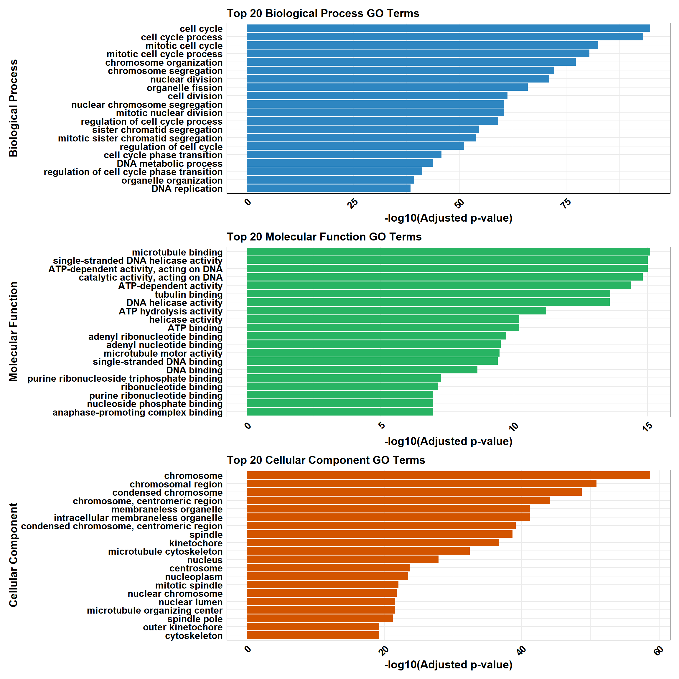
# Function for plotting top terms
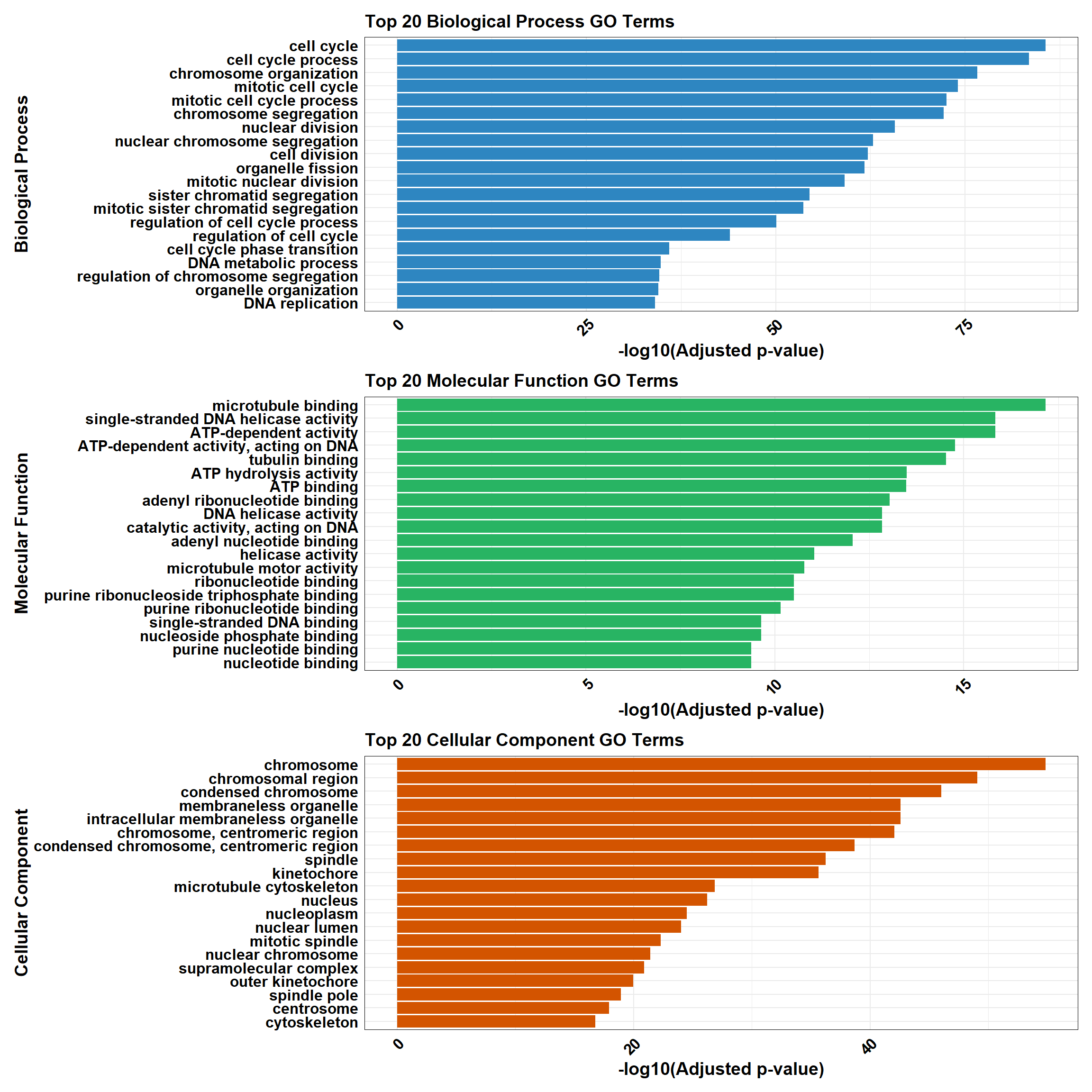
plot_gprofiler_results <- function(data, title, color) {
ggplot(data, aes(x = -log10(p.adjust), y = reorder(term_name, -log10(p.adjust)))) +
geom_bar(stat = "identity", fill = color) +
labs(
x = "-log10(Adjusted p-value)",
y = title,
title = paste("Top 20", title, "GO Terms")
) +
theme_minimal() +
theme(
axis.text.x = element_text(size = 12, face = "bold", colour = "black", angle = 45, hjust = 1),
axis.text.y = element_text(size = 12, face = "bold", colour = "black"),
axis.title.x = element_text(size = 14, face = "bold", colour = "black"),
axis.title.y = element_text(size = 14, face = "bold", colour = "black"),
plot.title = element_text(size = 14, face = "bold", colour = "black"),
panel.border = element_rect(colour = "black", fill = NA, size = 0.3)
)
}
# Check if there are enrichment terms to plot
if (nrow(combined_results) == 1 && combined_results$term_name == "No enriched terms") {
message("No enriched GO terms found for the input gene set.")
} else {
# Plot the top 20 terms for each category
plot_BP <- plot_gprofiler_results(top_BP, "Biological Process", "#2E86C1")
plot_MF <- plot_gprofiler_results(top_MF, "Molecular Function", "#28B463")
plot_CC <- plot_gprofiler_results(top_CC, "Cellular Component", "#D35400")
# Combine the plots using patchwork
combined_plot <- plot_BP / plot_MF / plot_CC
# Display the combined plot
combined_plot
}📌 CX vs VEH (0.1 and 3hr) Pathway Enrichment
# Load required libraries
library(clusterProfiler)
library(org.Hs.eg.db) # Required for enrichPathway
library(gprofiler2)
library(ggplot2)
library(dplyr)
library(patchwork)
library(ReactomePA)Warning: package 'ReactomePA' was built under R version 4.3.1# Function for ClusterProfiler Reactome & KEGG Analysis
process_clusterProfiler <- function(gene_set, background, category, color, y_title) {
# Perform enrichment based on the selected category
if (category == "Reactome") {
enrichment <- enrichPathway(
gene = gene_set,
organism = "human",
pvalueCutoff = 0.05,
pAdjustMethod = "BH",
universe = background
)
} else if (category == "KEGG") {
enrichment <- enrichKEGG(
gene = gene_set,
organism = "hsa",
pvalueCutoff = 0.05,
pAdjustMethod = "BH",
universe = background
)
}
# Check if enrichment results exist
if (is.null(enrichment) || nrow(as.data.frame(enrichment)) == 0) {
message(paste("No significant enrichment found for", category, "in ClusterProfiler"))
return(NULL)
}
# Convert results to tibble and process top 20 terms
enrichment_tibble <- as_tibble(as.data.frame(enrichment)) %>%
mutate(Category = category,
neglog = -log10(p.adjust)) %>% # Compute -log10(p.adjust)
arrange(desc(neglog)) %>%
slice_head(n = min(20, nrow(.))) # Ensure safe slicing
# Generate plot
plot <- ggplot(enrichment_tibble, aes(x = neglog, y = reorder(Description, neglog))) +
geom_bar(stat = "identity", fill = color) +
labs(x = "-log10(Adjusted p-value)",
y = y_title,
title = paste("Enriched", category, "Pathways")) +
theme_minimal() +
theme(
axis.text.x = element_text(size = 12, face = "bold", colour = "black", angle = 45, hjust = 1),
axis.text.y = element_text(size = 12, face = "bold", colour = "black"),
axis.title.x = element_text(size = 14, face = "bold", colour = "black"),
axis.title.y = element_text(size = 14, face = "bold", colour = "black"),
plot.title = element_text(size = 14, face = "bold", colour = "black")
)
return(plot)
}
# Function for gProfiler Reactome & KEGG Analysis
process_gprofiler <- function(gene_set, background, category, color, y_title) {
# Perform enrichment using gprofiler2
enrichment <- gost(
query = gene_set,
organism = "hsapiens",
user_threshold = 0.05,
correction_method = "fdr",
domain_scope = "custom",
custom_bg = background,
sources = category # Either "REAC" or "KEGG"
)
# Check if enrichment results exist
if (is.null(enrichment$result) || nrow(enrichment$result) == 0) {
message(paste("No significant enrichment found for", category, "in gProfiler"))
return(NULL)
}
# Convert results to tibble and process top 20 terms
enrichment_tibble <- enrichment$result %>%
as_tibble() %>%
mutate(Category = category,
neglog = -log10(p_value)) %>% # Compute -log10(p-value)
arrange(desc(neglog)) %>%
slice_head(n = min(20, nrow(.))) # Ensure safe slicing
# Generate plot
plot <- ggplot(enrichment_tibble, aes(x = neglog, y = reorder(term_name, neglog))) +
geom_bar(stat = "identity", fill = color) +
labs(x = "-log10(p-value)",
y = y_title,
title = paste("Enriched", category, "Pathways")) +
theme_minimal() +
theme(
axis.text.x = element_text(size = 12, face = "bold", colour = "black", angle = 45, hjust = 1),
axis.text.y = element_text(size = 12, face = "bold", colour = "black"),
axis.title.x = element_text(size = 14, face = "bold", colour = "black"),
axis.title.y = element_text(size = 14, face = "bold", colour = "black"),
plot.title = element_text(size = 14, face = "bold", colour = "black")
)
return(plot)
}
# Perform analysis for Reactome and KEGG using ClusterProfiler
cluster_reactome <- process_clusterProfiler(
gene_set = DEG1,
background = background,
category = "Reactome",
color = "#2E86C1",
y_title = "Reactome Pathways"
)
cluster_kegg <- process_clusterProfiler(
gene_set = DEG1,
background = background,
category = "KEGG",
color = "#28B463",
y_title = "KEGG Pathways"
)
# Combine Reactome and KEGG for ClusterProfiler
if (!is.null(cluster_reactome) && !is.null(cluster_kegg)) {
cluster_combined <- cluster_reactome / cluster_kegg
} else if (!is.null(cluster_reactome)) {
cluster_combined <- cluster_reactome
} else if (!is.null(cluster_kegg)) {
cluster_combined <- cluster_kegg
} else {
cluster_combined <- NULL
}
# Perform analysis for Reactome and KEGG using GProfiler
gprofiler_reactome <- process_gprofiler(
gene_set = DEG1,
background = background,
category = "REAC", # Corrected category for Reactome in gProfiler
color = "#D35400",
y_title = "Reactome Pathways"
)
gprofiler_kegg <- process_gprofiler(
gene_set = DEG1,
background = background,
category = "KEGG",
color = "#F39C12",
y_title = "KEGG Pathways"
)
# Combine Reactome and KEGG for GProfiler
if (!is.null(gprofiler_reactome) && !is.null(gprofiler_kegg)) {
gprofiler_combined <- gprofiler_reactome / gprofiler_kegg
} else if (!is.null(gprofiler_reactome)) {
gprofiler_combined <- gprofiler_reactome
} else if (!is.null(gprofiler_kegg)) {
gprofiler_combined <- gprofiler_kegg
} else {
gprofiler_combined <- NULL
}
# Display plots (if they are not NULL)
if (!is.null(cluster_combined)) print(cluster_combined)
if (!is.null(gprofiler_combined)) print(gprofiler_combined)📌 CX vs VEH (0.1 and 24hr)
📌 CX vs VEH (0.1 and 24hr) GO Enrichment Clusterprofiler
# Perform GO enrichment analysis for BP, MF, and CC
go_enrichment_BP <- enrichGO(gene = DEG2,
OrgDb = org.Hs.eg.db,
keyType = "ENTREZID",
universe = background,
ont = "BP",
pvalueCutoff = 0.05)
go_enrichment_MF <- enrichGO(gene = DEG2,
OrgDb = org.Hs.eg.db,
keyType = "ENTREZID",
universe = background,
ont = "MF",
pvalueCutoff = 0.05)
go_enrichment_CC <- enrichGO(gene = DEG2,
OrgDb = org.Hs.eg.db,
keyType = "ENTREZID",
universe = background,
ont = "CC",
pvalueCutoff = 0.05)
# Convert each enrichment result to a tibble, add a category column, and select top 20 terms
process_enrichment_tibble <- function(enrichment, category) {
if (is.null(enrichment) || nrow(as.data.frame(enrichment)) == 0) {
return(tibble(Description = "No enriched terms", neglog = 0, Category = category))
} else {
enrichment %>%
as_tibble() %>%
mutate(Category = category,
neglog = -log(p.adjust)) %>% # Add -log(p.adjust) column
arrange(desc(neglog)) %>% # Sort by -log(p.adjust)
slice(1:20) # Select top 20 terms
}
}
BP_Tibble <- process_enrichment_tibble(go_enrichment_BP, "Biological Process")
MF_Tibble <- process_enrichment_tibble(go_enrichment_MF, "Molecular Function")
CC_Tibble <- process_enrichment_tibble(go_enrichment_CC, "Cellular Component")
# Combine all tibbles
combined_GO_Tibble <- bind_rows(BP_Tibble, MF_Tibble, CC_Tibble)
# Function to generate enrichment plots
process_enrichment_plot <- function(tibble, title, color) {
ggplot(data = tibble, aes(x = neglog, y = reorder(Description, neglog))) +
geom_bar(stat = "identity", fill = color) +
labs(x = "-log(p-adjust)",
y = title,
title = paste("Top 20", title, "GO Terms")) +
theme_minimal() +
theme(
axis.text.x = element_text(size = 12, face = "bold", colour = "black", angle = 45, hjust = 1),
axis.text.y = element_text(size = 12, face = "bold", colour = "black"),
axis.title.x = element_text(size = 14, face = "bold", colour = "black"),
axis.title.y = element_text(size = 14, face = "bold", colour = "black"),
plot.title = element_text(size = 14, face = "bold", colour = "black"),
panel.border = element_rect(colour = "black", fill = NA, size = 0.3)
) +
xlim(c(0, max(tibble$neglog) + 1))
}
# Generate separate plots
plot_BP <- process_enrichment_plot(BP_Tibble, "Biological Process", "#2E86C1")
plot_MF <- process_enrichment_plot(MF_Tibble, "Molecular Function", "#28B463")
plot_CC <- process_enrichment_plot(CC_Tibble, "Cellular Component", "#D35400")

# Combine the plots using patchwork
combined_plot <- plot_BP / plot_MF / plot_CC

# Display the combined plot
combined_plot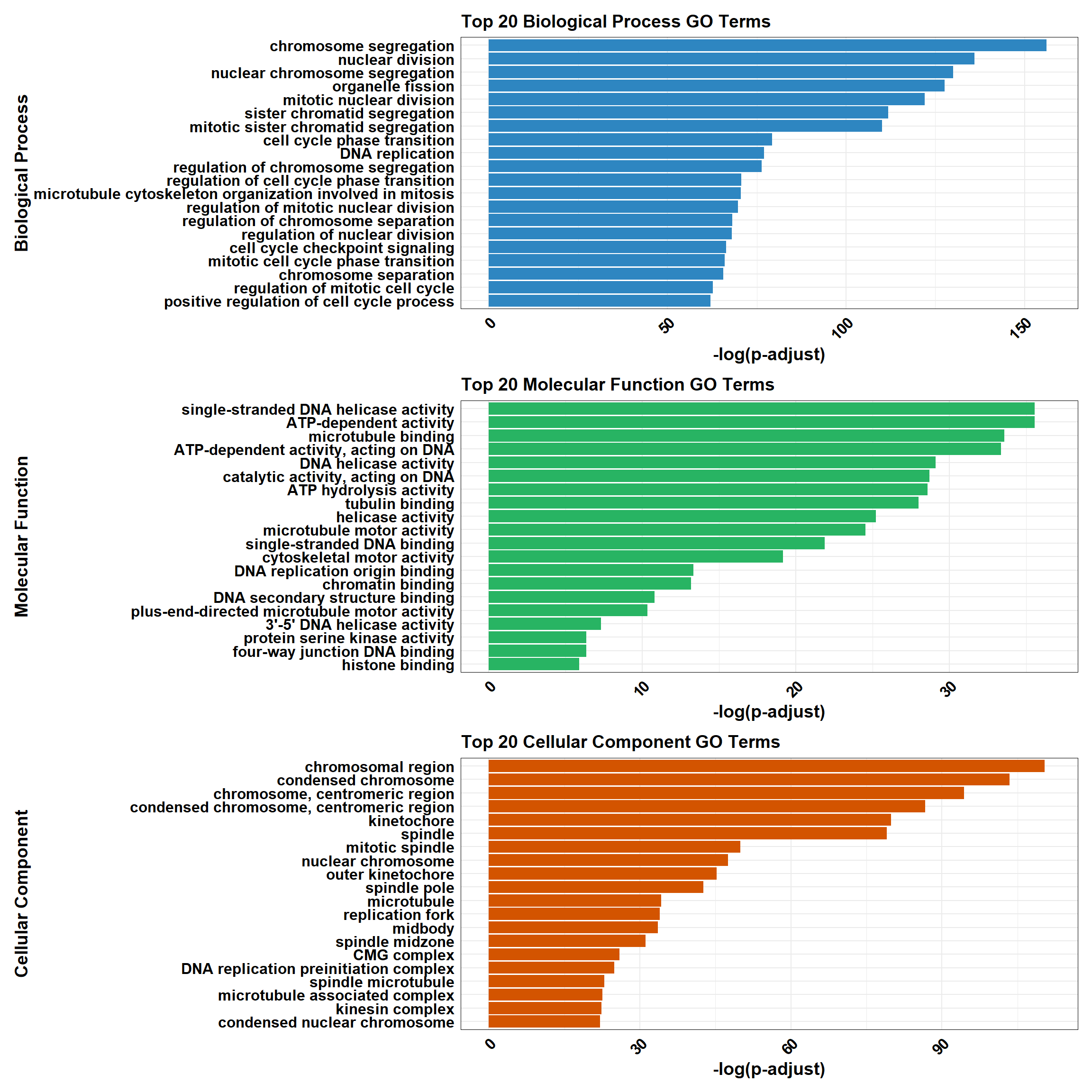
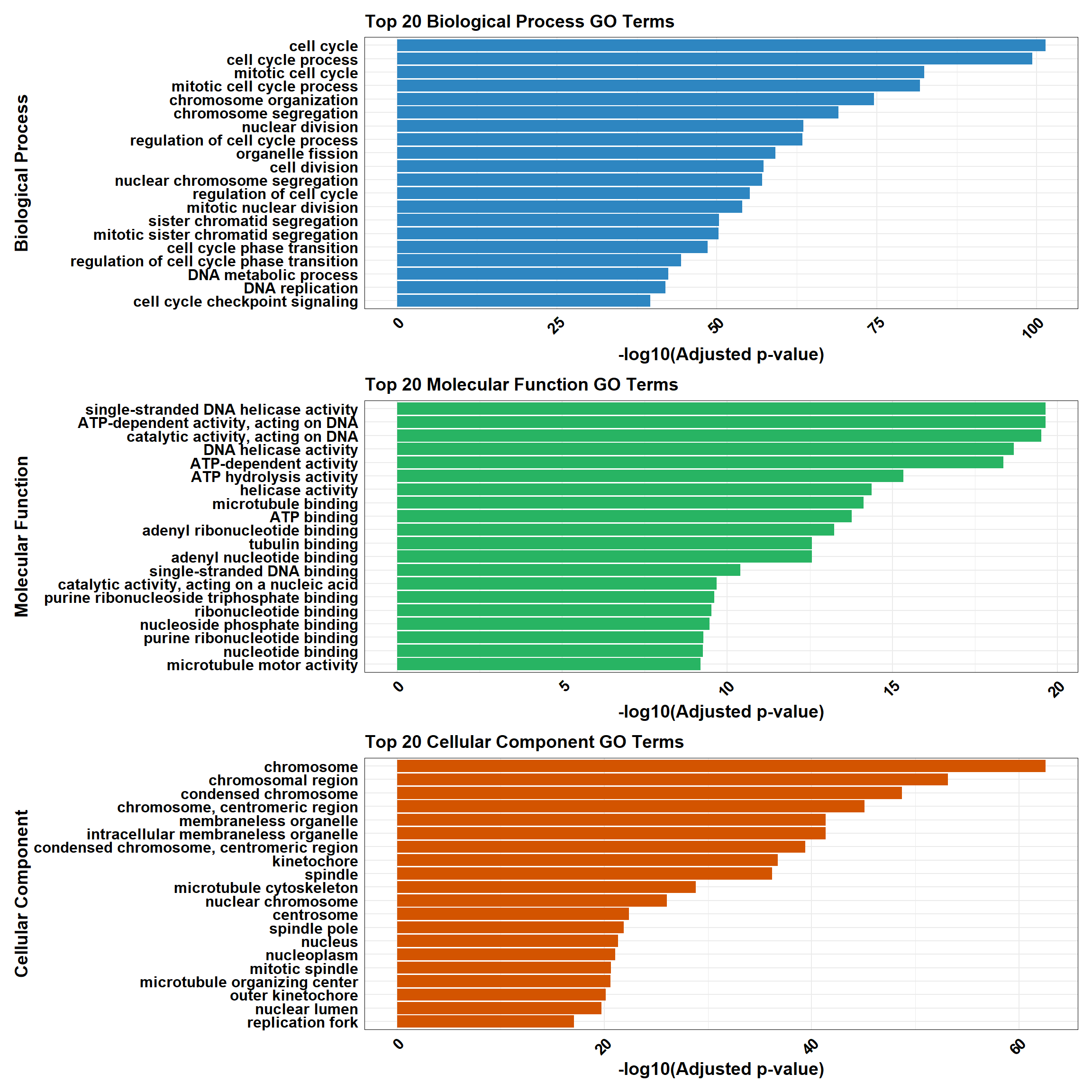
📌 CX vs VEH (0.1 and 24hr) GO Enrichment g:Profiler
# Load the gprofiler2 package
library(gprofiler2)
library(ggplot2)
library(dplyr)
library(patchwork)
# Perform GO enrichment analysis with gprofiler2
gost_results <- gost(
query = DEG2, # List of input genes (DEG1)
organism = "hsapiens", # Human organism
user_threshold = 0.05, # Adjusted p-value cutoff
correction_method = "fdr", # Multiple testing correction
domain_scope = "custom", # Use custom background
custom_bg = background, # Background set of genes
sources = c("GO:BP", "GO:MF", "GO:CC") # Analyze GO categories
)
# Check if enrichment results exist
if (is.null(gost_results$result) || nrow(gost_results$result) == 0) {
# If no enriched terms, create a placeholder dataframe
combined_results <- tibble(
term_name = "No enriched terms",
p.adjust = NA,
source = "N/A",
Category = "N/A"
)
} else {
# Convert results to a data frame
gost_results_df <- gost_results$result
# Add a column for adjusted p-value
gost_results_df <- gost_results_df %>%
rename(p.adjust = p_value)
# Separate results for BP, MF, and CC
BP_results <- gost_results_df %>%
filter(source == "GO:BP") %>%
mutate(Category = "Biological Process")
MF_results <- gost_results_df %>%
filter(source == "GO:MF") %>%
mutate(Category = "Molecular Function")
CC_results <- gost_results_df %>%
filter(source == "GO:CC") %>%
mutate(Category = "Cellular Component")
# Select the top 20 terms by adjusted p-value for each category
top_BP <- BP_results %>%
arrange(p.adjust) %>%
slice_head(n = 20)
top_MF <- MF_results %>%
arrange(p.adjust) %>%
slice_head(n = 20)
top_CC <- CC_results %>%
arrange(p.adjust) %>%
slice_head(n = 20)
# Combine all categories
combined_results <- bind_rows(top_BP, top_MF, top_CC)
}
# Ensure all columns are atomic types for CSV export
combined_results_clean <- combined_results %>%
mutate(across(everything(), ~ if (is.list(.)) sapply(., toString) else .))
# Function for plotting top terms
plot_gprofiler_results <- function(data, title, color) {
ggplot(data, aes(x = -log10(p.adjust), y = reorder(term_name, -log10(p.adjust)))) +
geom_bar(stat = "identity", fill = color) +
labs(
x = "-log10(Adjusted p-value)",
y = title,
title = paste("Top 20", title, "GO Terms")
) +
theme_minimal() +
theme(
axis.text.x = element_text(size = 12, face = "bold", colour = "black", angle = 45, hjust = 1),
axis.text.y = element_text(size = 12, face = "bold", colour = "black"),
axis.title.x = element_text(size = 14, face = "bold", colour = "black"),
axis.title.y = element_text(size = 14, face = "bold", colour = "black"),
plot.title = element_text(size = 14, face = "bold", colour = "black"),
panel.border = element_rect(colour = "black", fill = NA, size = 0.3)
)
}
# Check if there are enrichment terms to plot
if (nrow(combined_results) == 1 && combined_results$term_name == "No enriched terms") {
message("No enriched GO terms found for the input gene set.")
} else {
# Plot the top 20 terms for each category
plot_BP <- plot_gprofiler_results(top_BP, "Biological Process", "#2E86C1")
plot_MF <- plot_gprofiler_results(top_MF, "Molecular Function", "#28B463")
plot_CC <- plot_gprofiler_results(top_CC, "Cellular Component", "#D35400")
# Combine the plots using patchwork
combined_plot <- plot_BP / plot_MF / plot_CC
# Display the combined plot
combined_plot
}
📌 CX vs VEH (0.1 and 24hr) Pathway Enrichment
# Load required libraries
library(clusterProfiler)
library(org.Hs.eg.db) # Required for enrichPathway
library(gprofiler2)
library(ggplot2)
library(dplyr)
library(patchwork)
library(ReactomePA)
# Function for ClusterProfiler Reactome & KEGG Analysis
process_clusterProfiler <- function(gene_set, background, category, color, y_title) {
# Perform enrichment based on the selected category
if (category == "Reactome") {
enrichment <- enrichPathway(
gene = gene_set,
organism = "human",
pvalueCutoff = 0.05,
pAdjustMethod = "BH",
universe = background
)
} else if (category == "KEGG") {
enrichment <- enrichKEGG(
gene = gene_set,
organism = "hsa",
pvalueCutoff = 0.05,
pAdjustMethod = "BH",
universe = background
)
}
# Check if enrichment results exist
if (is.null(enrichment) || nrow(as.data.frame(enrichment)) == 0) {
message(paste("No significant enrichment found for", category, "in ClusterProfiler"))
return(NULL)
}
# Convert results to tibble and process top 20 terms
enrichment_tibble <- as_tibble(as.data.frame(enrichment)) %>%
mutate(Category = category,
neglog = -log10(p.adjust)) %>% # Compute -log10(p.adjust)
arrange(desc(neglog)) %>%
slice_head(n = min(20, nrow(.))) # Ensure safe slicing
# Generate plot
plot <- ggplot(enrichment_tibble, aes(x = neglog, y = reorder(Description, neglog))) +
geom_bar(stat = "identity", fill = color) +
labs(x = "-log10(Adjusted p-value)",
y = y_title,
title = paste("Enriched", category, "Pathways")) +
theme_minimal() +
theme(
axis.text.x = element_text(size = 12, face = "bold", colour = "black", angle = 45, hjust = 1),
axis.text.y = element_text(size = 12, face = "bold", colour = "black"),
axis.title.x = element_text(size = 14, face = "bold", colour = "black"),
axis.title.y = element_text(size = 14, face = "bold", colour = "black"),
plot.title = element_text(size = 14, face = "bold", colour = "black")
)
return(plot)
}
# Function for gProfiler Reactome & KEGG Analysis
process_gprofiler <- function(gene_set, background, category, color, y_title) {
# Perform enrichment using gprofiler2
enrichment <- gost(
query = gene_set,
organism = "hsapiens",
user_threshold = 0.05,
correction_method = "fdr",
domain_scope = "custom",
custom_bg = background,
sources = category # Either "REAC" or "KEGG"
)
# Check if enrichment results exist
if (is.null(enrichment$result) || nrow(enrichment$result) == 0) {
message(paste("No significant enrichment found for", category, "in gProfiler"))
return(NULL)
}
# Convert results to tibble and process top 20 terms
enrichment_tibble <- enrichment$result %>%
as_tibble() %>%
mutate(Category = category,
neglog = -log10(p_value)) %>% # Compute -log10(p-value)
arrange(desc(neglog)) %>%
slice_head(n = min(20, nrow(.))) # Ensure safe slicing
# Generate plot
plot <- ggplot(enrichment_tibble, aes(x = neglog, y = reorder(term_name, neglog))) +
geom_bar(stat = "identity", fill = color) +
labs(x = "-log10(p-value)",
y = y_title,
title = paste("Enriched", category, "Pathways")) +
theme_minimal() +
theme(
axis.text.x = element_text(size = 12, face = "bold", colour = "black", angle = 45, hjust = 1),
axis.text.y = element_text(size = 12, face = "bold", colour = "black"),
axis.title.x = element_text(size = 14, face = "bold", colour = "black"),
axis.title.y = element_text(size = 14, face = "bold", colour = "black"),
plot.title = element_text(size = 14, face = "bold", colour = "black")
)
return(plot)
}
# Perform analysis for Reactome and KEGG using ClusterProfiler
cluster_reactome <- process_clusterProfiler(
gene_set = DEG2,
background = background,
category = "Reactome",
color = "#2E86C1",
y_title = "Reactome Pathways"
)
cluster_kegg <- process_clusterProfiler(
gene_set = DEG2,
background = background,
category = "KEGG",
color = "#28B463",
y_title = "KEGG Pathways"
)
# Combine Reactome and KEGG for ClusterProfiler
if (!is.null(cluster_reactome) && !is.null(cluster_kegg)) {
cluster_combined <- cluster_reactome / cluster_kegg
} else if (!is.null(cluster_reactome)) {
cluster_combined <- cluster_reactome
} else if (!is.null(cluster_kegg)) {
cluster_combined <- cluster_kegg
} else {
cluster_combined <- NULL
}
# Perform analysis for Reactome and KEGG using GProfiler
gprofiler_reactome <- process_gprofiler(
gene_set = DEG2,
background = background,
category = "REAC", # Corrected category for Reactome in gProfiler
color = "#D35400",
y_title = "Reactome Pathways"
)
gprofiler_kegg <- process_gprofiler(
gene_set = DEG2,
background = background,
category = "KEGG",
color = "#F39C12",
y_title = "KEGG Pathways"
)
# Combine Reactome and KEGG for GProfiler
if (!is.null(gprofiler_reactome) && !is.null(gprofiler_kegg)) {
gprofiler_combined <- gprofiler_reactome / gprofiler_kegg
} else if (!is.null(gprofiler_reactome)) {
gprofiler_combined <- gprofiler_reactome
} else if (!is.null(gprofiler_kegg)) {
gprofiler_combined <- gprofiler_kegg
} else {
gprofiler_combined <- NULL
}
# Display plots (if they are not NULL)
if (!is.null(cluster_combined)) print(cluster_combined)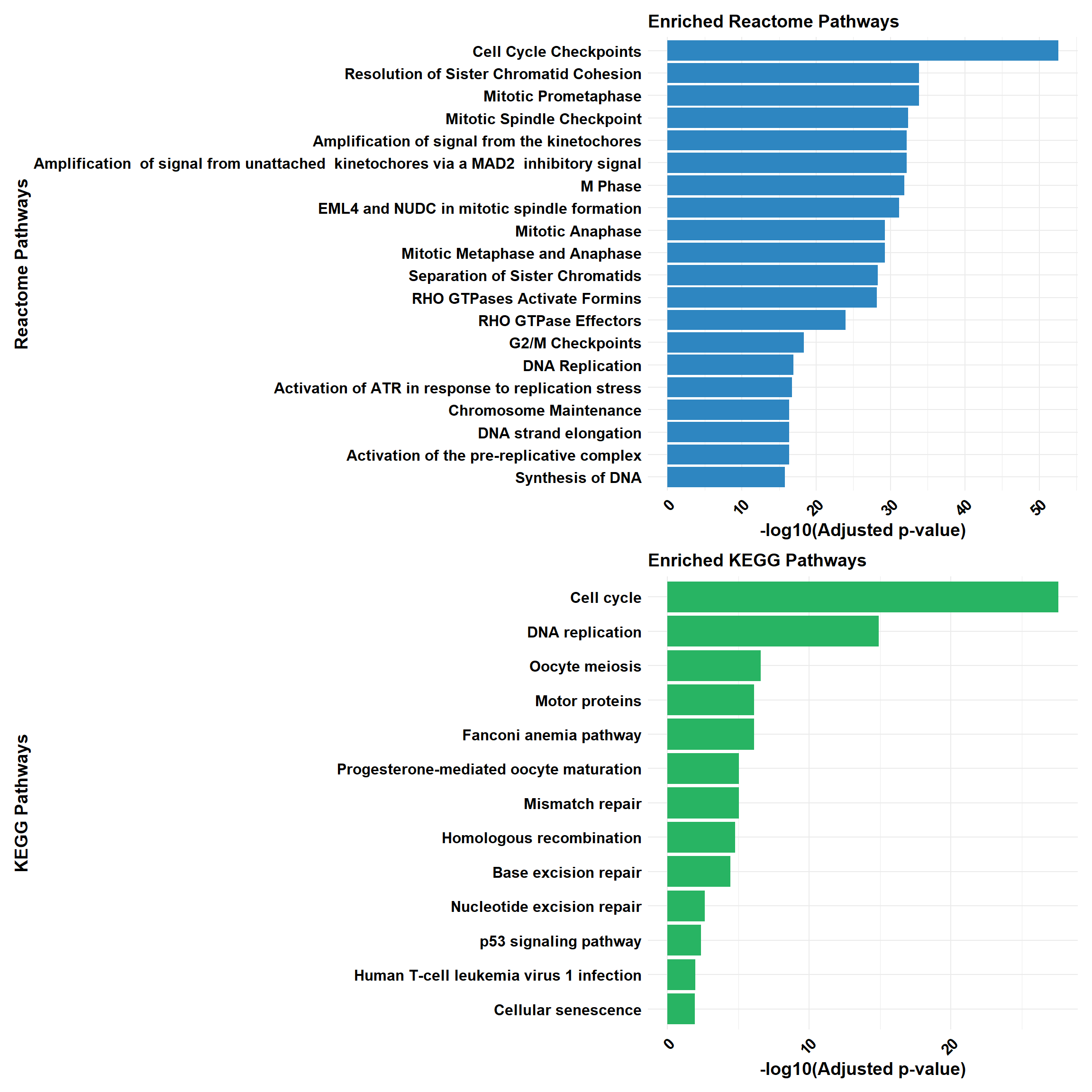
if (!is.null(gprofiler_combined)) print(gprofiler_combined)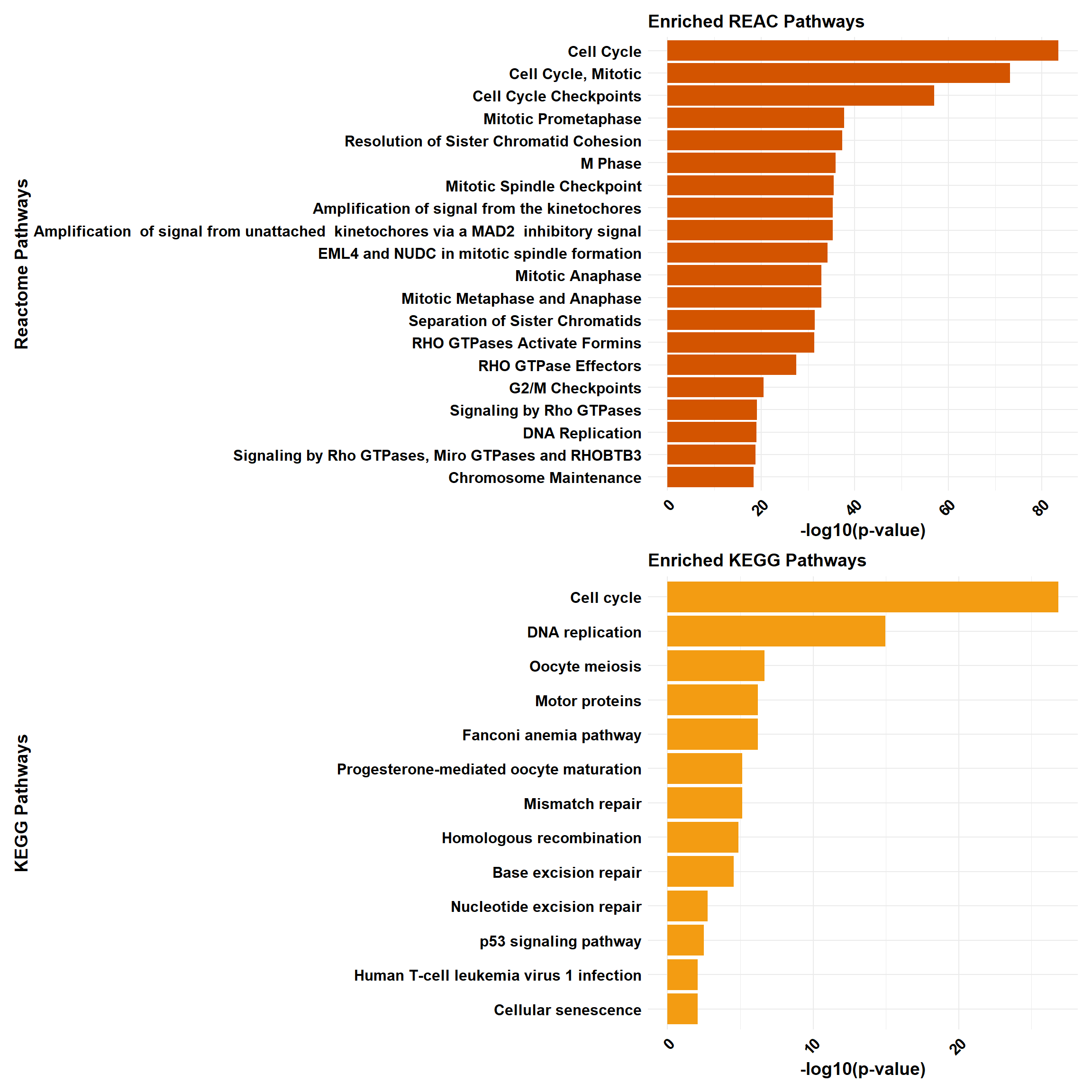
📌 CX vs VEH (0.1 and 48hr)
📌 CX vs VEH (0.1 and 48hr) GO Enrichment Clusterprofiler
# Perform GO enrichment analysis for BP, MF, and CC
go_enrichment_BP <- enrichGO(gene = DEG3,
                             OrgDb = org.Hs.eg.db,
                             keyType = "ENTREZID",
                             universe = background,
                             ont = "BP",
                             pvalueCutoff = 0.05)

go_enrichment_MF <- enrichGO(gene = DEG3,
                             OrgDb = org.Hs.eg.db,
                             keyType = "ENTREZID",
                             universe = background,
                             ont = "MF",
                             pvalueCutoff = 0.05)

go_enrichment_CC <- enrichGO(gene = DEG3,
                             OrgDb = org.Hs.eg.db,
                             keyType = "ENTREZID",
                             universe = background,
                             ont = "CC",
                             pvalueCutoff = 0.05)

# Convert each enrichment result to a tibble, add a category column, and select top 20 terms
process_enrichment_tibble <- function(enrichment, category) {
  if (is.null(enrichment) || nrow(as.data.frame(enrichment)) == 0) {
    return(tibble(Description = "No enriched terms", neglog = 0, Category = category))
  } else {
    enrichment %>%
      as_tibble() %>%
      mutate(Category = category,
             neglog = -log(p.adjust)) %>% # Add -log(p.adjust) column
      arrange(desc(neglog)) %>%          # Sort by -log(p.adjust)
      slice(1:20)                        # Select top 20 terms
  }
}

BP_Tibble <- process_enrichment_tibble(go_enrichment_BP, "Biological Process")
MF_Tibble <- process_enrichment_tibble(go_enrichment_MF, "Molecular Function")
CC_Tibble <- process_enrichment_tibble(go_enrichment_CC, "Cellular Component")

# Combine all tibbles
combined_GO_Tibble <- bind_rows(BP_Tibble, MF_Tibble, CC_Tibble)
# Function to generate enrichment plots
process_enrichment_plot <- function(tibble, title, color) {
  ggplot(data = tibble, aes(x = neglog, y = reorder(Description, neglog))) +
    geom_bar(stat = "identity", fill = color) +
    labs(x = "-log(p-adjust)",
         y = title,
         title = paste("Top 20", title, "GO Terms")) +
    theme_minimal() +
    theme(
      axis.text.x = element_text(size = 12, face = "bold", colour = "black", angle = 45, hjust = 1),
      axis.text.y = element_text(size = 12, face = "bold", colour = "black"),
      axis.title.x = element_text(size = 14, face = "bold", colour = "black"),
      axis.title.y = element_text(size = 14, face = "bold", colour = "black"),
      plot.title = element_text(size = 14, face = "bold", colour = "black"),
      panel.border = element_rect(colour = "black", fill = NA, size = 0.3)
    ) +
    xlim(c(0, max(tibble$neglog) + 1))
}

# Generate separate plots
plot_BP <- process_enrichment_plot(BP_Tibble, "Biological Process", "#2E86C1")
plot_MF <- process_enrichment_plot(MF_Tibble, "Molecular Function", "#28B463")
plot_CC <- process_enrichment_plot(CC_Tibble, "Cellular Component", "#D35400")

# Combine the plots using patchwork
combined_plot <- plot_BP / plot_MF / plot_CC

# Display the combined plot
combined_plot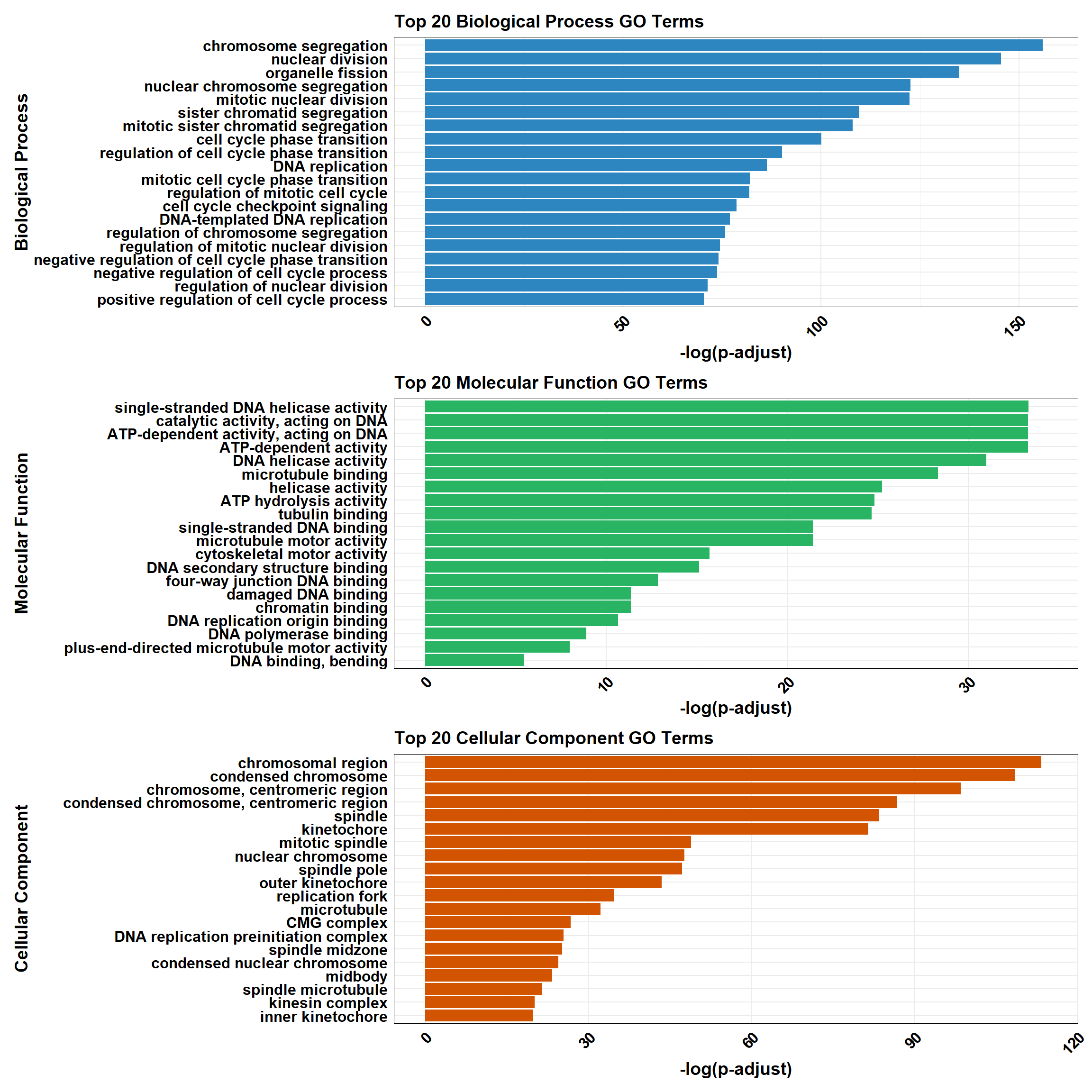
📌 CX vs VEH (0.1 and 48hr) GO Enrichment g:Profiler
# Load the gprofiler2 package
library(gprofiler2)
library(ggplot2)
library(dplyr)
library(patchwork)

# Perform GO enrichment analysis with gprofiler2
gost_results <- gost(
  query = DEG3,
  organism = "hsapiens",   # Human organism
  user_threshold = 0.05,   # Adjusted p-value cutoff
  correction_method = "fdr", # Multiple testing correction
  domain_scope = "custom", # Use custom background
  custom_bg = background,    # Background set of genes
  sources = c("GO:BP", "GO:MF", "GO:CC") # Analyze GO categories
)

# Check if enrichment results exist
if (is.null(gost_results$result) || nrow(gost_results$result) == 0) {
  # If no enriched terms, create a placeholder dataframe
  combined_results <- tibble(
    term_name = "No enriched terms",
    p.adjust = NA,
    source = "N/A",
    Category = "N/A"
  )
} else {
  # Convert results to a data frame
  gost_results_df <- gost_results$result

  # Add a column for adjusted p-value
  gost_results_df <- gost_results_df %>%
    rename(p.adjust = p_value)

  # Separate results for BP, MF, and CC
  BP_results <- gost_results_df %>%
    filter(source == "GO:BP") %>%
    mutate(Category = "Biological Process")

  MF_results <- gost_results_df %>%
    filter(source == "GO:MF") %>%
    mutate(Category = "Molecular Function")

  CC_results <- gost_results_df %>%
    filter(source == "GO:CC") %>%
    mutate(Category = "Cellular Component")

  # Select the top 20 terms by adjusted p-value for each category
  top_BP <- BP_results %>%
    arrange(p.adjust) %>%
    slice_head(n = 20)

  top_MF <- MF_results %>%
    arrange(p.adjust) %>%
    slice_head(n = 20)

  top_CC <- CC_results %>%
    arrange(p.adjust) %>%
    slice_head(n = 20)

  # Combine all categories
  combined_results <- bind_rows(top_BP, top_MF, top_CC)
}

# Ensure all columns are atomic types for CSV export
combined_results_clean <- combined_results %>%
  mutate(across(everything(), ~ if (is.list(.)) sapply(., toString) else .))

# Function for plotting top terms
plot_gprofiler_results <- function(data, title, color) {
  ggplot(data, aes(x = -log10(p.adjust), y = reorder(term_name, -log10(p.adjust)))) +
    geom_bar(stat = "identity", fill = color) +
    labs(
      x = "-log10(Adjusted p-value)",
      y = title,
      title = paste("Top 20", title, "GO Terms")
    ) +
    theme_minimal() +
    theme(
      axis.text.x = element_text(size = 12, face = "bold", colour = "black", angle = 45, hjust = 1),
      axis.text.y = element_text(size = 12, face = "bold", colour = "black"),
      axis.title.x = element_text(size = 14, face = "bold", colour = "black"),
      axis.title.y = element_text(size = 14, face = "bold", colour = "black"),
      plot.title = element_text(size = 14, face = "bold", colour = "black"),
      panel.border = element_rect(colour = "black", fill = NA, size = 0.3)
    )
}

# Check if there are enrichment terms to plot
if (nrow(combined_results) == 1 && combined_results$term_name == "No enriched terms") {
  message("No enriched GO terms found for the input gene set.")
} else {
  # Plot the top 20 terms for each category
  plot_BP <- plot_gprofiler_results(top_BP, "Biological Process", "#2E86C1")
  plot_MF <- plot_gprofiler_results(top_MF, "Molecular Function", "#28B463")
  plot_CC <- plot_gprofiler_results(top_CC, "Cellular Component", "#D35400")

  # Combine the plots using patchwork
  combined_plot <- plot_BP / plot_MF / plot_CC

  # Display the combined plot
  combined_plot
}
📌 CX vs VEH (0.1 and 48hr) Pathway Enrichment
# Load required libraries
library(clusterProfiler)
library(org.Hs.eg.db) # Required for enrichPathway
library(gprofiler2)
library(ggplot2)
library(dplyr)
library(patchwork)
library(ReactomePA)

# Function for ClusterProfiler Reactome & KEGG Analysis
process_clusterProfiler <- function(gene_set, background, category, color, y_title) {
  # Perform enrichment based on the selected category
  if (category == "Reactome") {
    enrichment <- enrichPathway(
      gene = gene_set,
      organism = "human",
      pvalueCutoff = 0.05,
      pAdjustMethod = "BH",
      universe = background
    )
  } else if (category == "KEGG") {
    enrichment <- enrichKEGG(
      gene = gene_set,
      organism = "hsa",
      pvalueCutoff = 0.05,
      pAdjustMethod = "BH",
      universe = background
    )
  }

  # Check if enrichment results exist
  if (is.null(enrichment) || nrow(as.data.frame(enrichment)) == 0) {
    message(paste("No significant enrichment found for", category, "in ClusterProfiler"))
    return(NULL)
  }

  # Convert results to tibble and process top 20 terms
  enrichment_tibble <- as_tibble(as.data.frame(enrichment)) %>%
    mutate(Category = category,
           neglog = -log10(p.adjust)) %>%  # Compute -log10(p.adjust)
    arrange(desc(neglog)) %>%
    slice_head(n = min(20, nrow(.)))  # Ensure safe slicing

  # Generate plot
  plot <- ggplot(enrichment_tibble, aes(x = neglog, y = reorder(Description, neglog))) +
    geom_bar(stat = "identity", fill = color) +
    labs(x = "-log10(Adjusted p-value)",
         y = y_title,
         title = paste("Enriched", category, "Pathways")) +
    theme_minimal() +
    theme(
      axis.text.x = element_text(size = 12, face = "bold", colour = "black", angle = 45, hjust = 1),
      axis.text.y = element_text(size = 12, face = "bold", colour = "black"),
      axis.title.x = element_text(size = 14, face = "bold", colour = "black"),
      axis.title.y = element_text(size = 14, face = "bold", colour = "black"),
      plot.title = element_text(size = 14, face = "bold", colour = "black")
    )

  return(plot)
}

# Function for gProfiler Reactome & KEGG Analysis
process_gprofiler <- function(gene_set, background, category, color, y_title) {
  # Perform enrichment using gprofiler2
  enrichment <- gost(
    query = gene_set,
    organism = "hsapiens",
    user_threshold = 0.05,
    correction_method = "fdr",
    domain_scope = "custom",
    custom_bg = background,
    sources = category # Either "REAC" or "KEGG"
  )

  # Check if enrichment results exist
  if (is.null(enrichment$result) || nrow(enrichment$result) == 0) {
    message(paste("No significant enrichment found for", category, "in gProfiler"))
    return(NULL)
  }

  # Convert results to tibble and process top 20 terms
  enrichment_tibble <- enrichment$result %>%
    as_tibble() %>%
    mutate(Category = category,
           neglog = -log10(p_value)) %>%  # Compute -log10(p-value)
    arrange(desc(neglog)) %>%
    slice_head(n = min(20, nrow(.)))  # Ensure safe slicing

  # Generate plot
  plot <- ggplot(enrichment_tibble, aes(x = neglog, y = reorder(term_name, neglog))) +
    geom_bar(stat = "identity", fill = color) +
    labs(x = "-log10(p-value)",
         y = y_title,
         title = paste("Enriched", category, "Pathways")) +
    theme_minimal() +
    theme(
      axis.text.x = element_text(size = 12, face = "bold", colour = "black", angle = 45, hjust = 1),
      axis.text.y = element_text(size = 12, face = "bold", colour = "black"),
      axis.title.x = element_text(size = 14, face = "bold", colour = "black"),
      axis.title.y = element_text(size = 14, face = "bold", colour = "black"),
      plot.title = element_text(size = 14, face = "bold", colour = "black")
    )

  return(plot)
}

# Perform analysis for Reactome and KEGG using ClusterProfiler
cluster_reactome <- process_clusterProfiler(
  gene_set = DEG3,
  background = background,
  category = "Reactome",
  color = "#2E86C1",
  y_title = "Reactome Pathways"
)

cluster_kegg <- process_clusterProfiler(
  gene_set = DEG3,
  background = background,
  category = "KEGG",
  color = "#28B463",
  y_title = "KEGG Pathways"
)

# Combine Reactome and KEGG for ClusterProfiler
if (!is.null(cluster_reactome) && !is.null(cluster_kegg)) {
  cluster_combined <- cluster_reactome / cluster_kegg
} else if (!is.null(cluster_reactome)) {
  cluster_combined <- cluster_reactome
} else if (!is.null(cluster_kegg)) {
  cluster_combined <- cluster_kegg
} else {
  cluster_combined <- NULL
}

# Perform analysis for Reactome and KEGG using GProfiler
gprofiler_reactome <- process_gprofiler(
  gene_set = DEG3,
  background = background,
  category = "REAC",  # Corrected category for Reactome in gProfiler
  color = "#D35400",
  y_title = "Reactome Pathways"
)

gprofiler_kegg <- process_gprofiler(
  gene_set = DEG3,
  background = background,
  category = "KEGG",
  color = "#F39C12",
  y_title = "KEGG Pathways"
)

# Combine Reactome and KEGG for GProfiler
if (!is.null(gprofiler_reactome) && !is.null(gprofiler_kegg)) {
  gprofiler_combined <- gprofiler_reactome / gprofiler_kegg
} else if (!is.null(gprofiler_reactome)) {
  gprofiler_combined <- gprofiler_reactome
} else if (!is.null(gprofiler_kegg)) {
  gprofiler_combined <- gprofiler_kegg
} else {
  gprofiler_combined <- NULL
}

# Display plots (if they are not NULL)
if (!is.null(cluster_combined)) print(cluster_combined)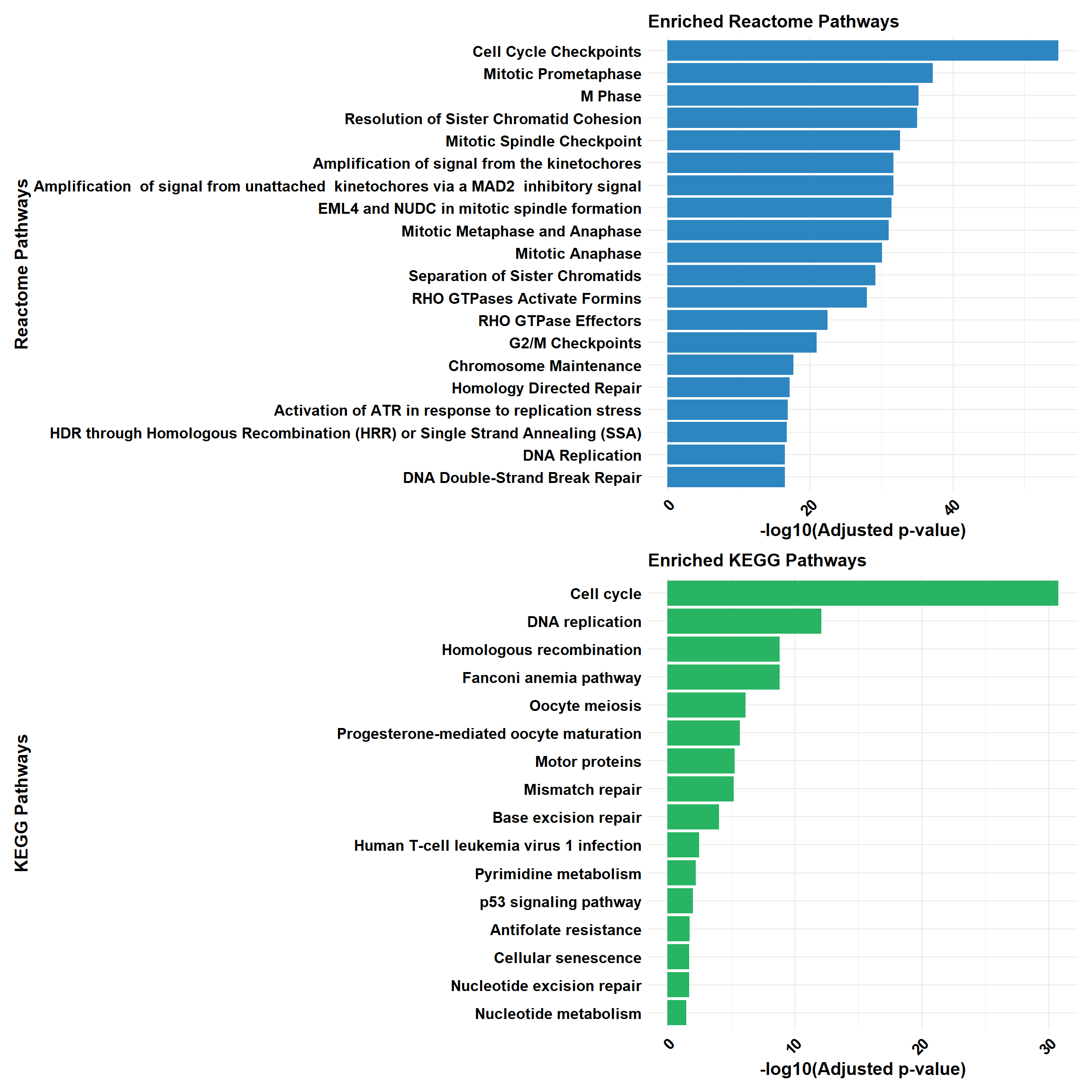
if (!is.null(gprofiler_combined)) print(gprofiler_combined)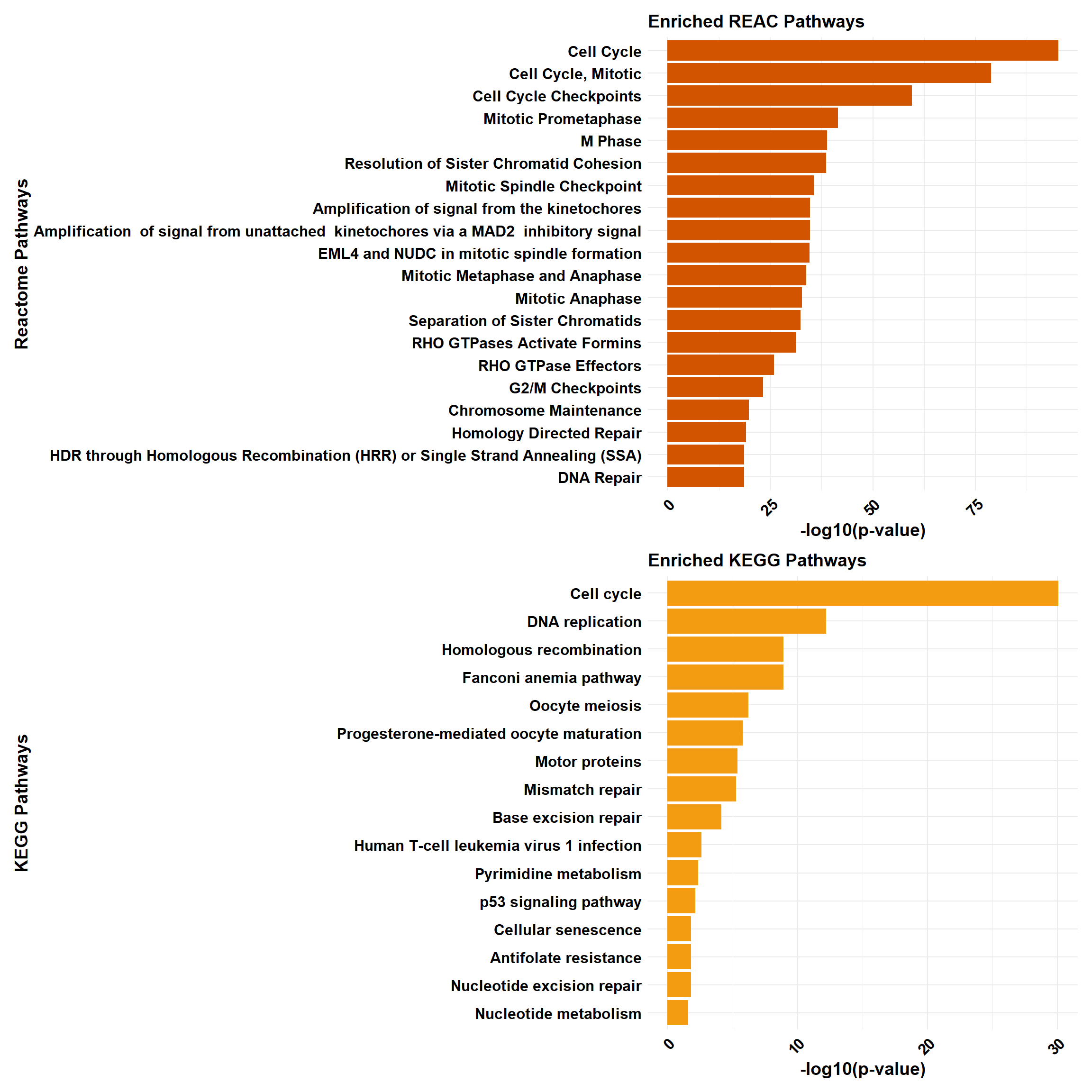
📌 CX vs VEH (0.5 and 3hr)
📌 CX vs VEH (0.5 and 3hr) GO Enrichment Clusterprofiler
# Perform GO enrichment analysis for BP, MF, and CC
go_enrichment_BP <- enrichGO(gene = DEG4,
                             OrgDb = org.Hs.eg.db,
                             keyType = "ENTREZID",
                             universe = background,
                             ont = "BP",
                             pvalueCutoff = 0.05)

go_enrichment_MF <- enrichGO(gene = DEG4,
                             OrgDb = org.Hs.eg.db,
                             keyType = "ENTREZID",
                             universe = background,
                             ont = "MF",
                             pvalueCutoff = 0.05)

go_enrichment_CC <- enrichGO(gene = DEG4,
                             OrgDb = org.Hs.eg.db,
                             keyType = "ENTREZID",
                             universe = background,
                             ont = "CC",
                             pvalueCutoff = 0.05)

# Convert each enrichment result to a tibble, add a category column, and select top 20 terms
process_enrichment_tibble <- function(enrichment, category) {
  if (is.null(enrichment) || nrow(as.data.frame(enrichment)) == 0) {
    return(tibble(Description = "No enriched terms", neglog = 0, Category = category))
  } else {
    enrichment %>%
      as_tibble() %>%
      mutate(Category = category,
             neglog = -log(p.adjust)) %>% # Add -log(p.adjust) column
      arrange(desc(neglog)) %>%          # Sort by -log(p.adjust)
      slice(1:20)                        # Select top 20 terms
  }
}

BP_Tibble <- process_enrichment_tibble(go_enrichment_BP, "Biological Process")
MF_Tibble <- process_enrichment_tibble(go_enrichment_MF, "Molecular Function")
CC_Tibble <- process_enrichment_tibble(go_enrichment_CC, "Cellular Component")

# Combine all tibbles
combined_GO_Tibble <- bind_rows(BP_Tibble, MF_Tibble, CC_Tibble)
# Function to generate enrichment plots
process_enrichment_plot <- function(tibble, title, color) {
  ggplot(data = tibble, aes(x = neglog, y = reorder(Description, neglog))) +
    geom_bar(stat = "identity", fill = color) +
    labs(x = "-log(p-adjust)",
         y = title,
         title = paste("Top 20", title, "GO Terms")) +
    theme_minimal() +
    theme(
      axis.text.x = element_text(size = 12, face = "bold", colour = "black", angle = 45, hjust = 1),
      axis.text.y = element_text(size = 12, face = "bold", colour = "black"),
      axis.title.x = element_text(size = 14, face = "bold", colour = "black"),
      axis.title.y = element_text(size = 14, face = "bold", colour = "black"),
      plot.title = element_text(size = 14, face = "bold", colour = "black"),
      panel.border = element_rect(colour = "black", fill = NA, size = 0.3)
    ) +
    xlim(c(0, max(tibble$neglog) + 1))
}

# Generate separate plots
plot_BP <- process_enrichment_plot(BP_Tibble, "Biological Process", "#2E86C1")
plot_MF <- process_enrichment_plot(MF_Tibble, "Molecular Function", "#28B463")
plot_CC <- process_enrichment_plot(CC_Tibble, "Cellular Component", "#D35400")

# Combine the plots using patchwork
combined_plot <- plot_BP / plot_MF / plot_CC

# Display the combined plot
combined_plot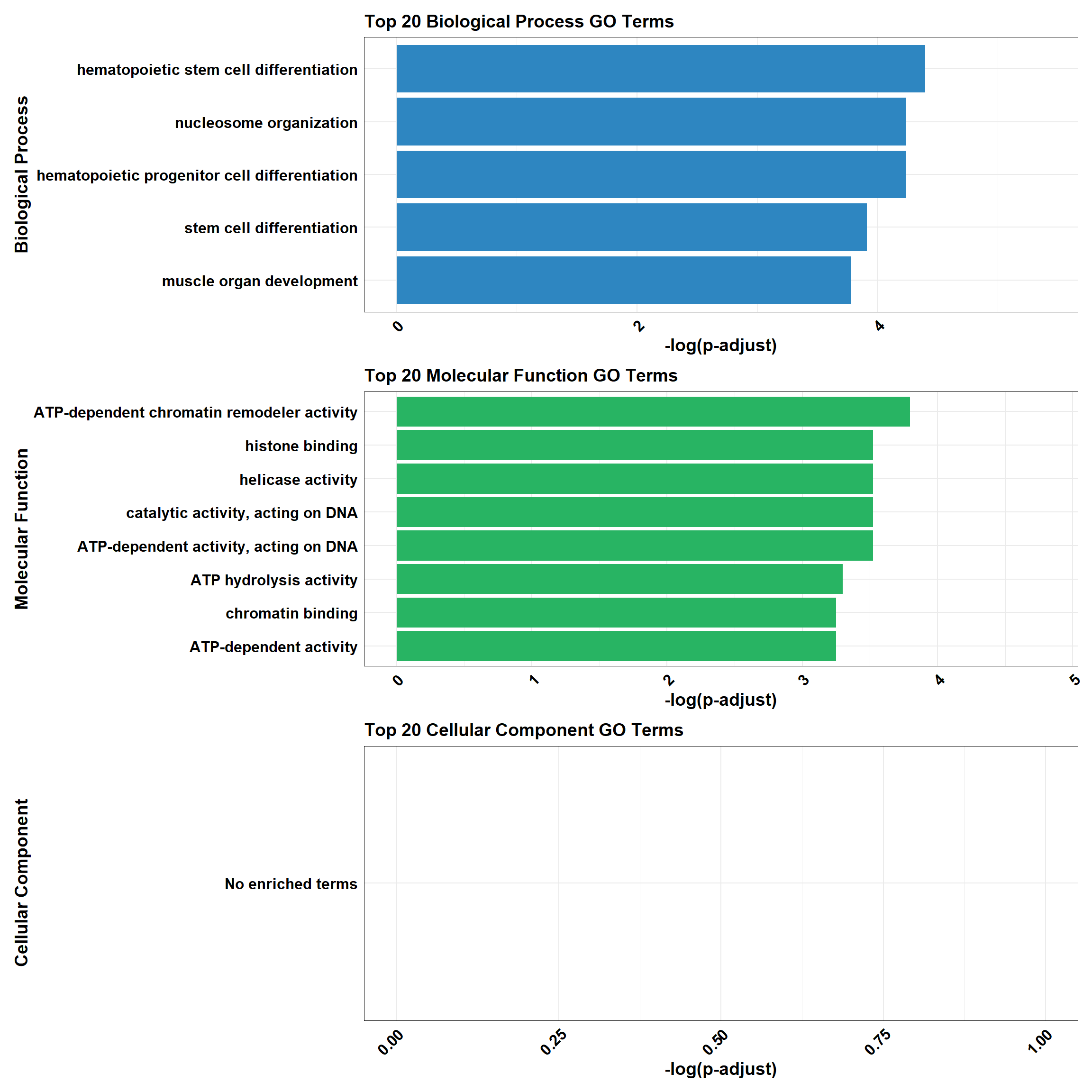
📌 CX vs VEH (0.5 and 3hr) GO Enrichment g:Profiler
# Load the gprofiler2 package
library(gprofiler2)
library(ggplot2)
library(dplyr)
library(patchwork)

# Perform GO enrichment analysis with gprofiler2
gost_results <- gost(
  query = DEG4,
  organism = "hsapiens",   # Human organism
  user_threshold = 0.05,   # Adjusted p-value cutoff
  correction_method = "fdr", # Multiple testing correction
  domain_scope = "custom", # Use custom background
  custom_bg = background,    # Background set of genes
  sources = c("GO:BP", "GO:MF", "GO:CC") # Analyze GO categories
)

# Check if enrichment results exist
if (is.null(gost_results$result) || nrow(gost_results$result) == 0) {
  # If no enriched terms, create a placeholder dataframe
  combined_results <- tibble(
    term_name = "No enriched terms",
    p.adjust = NA,
    source = "N/A",
    Category = "N/A"
  )
} else {
  # Convert results to a data frame
  gost_results_df <- gost_results$result

  # Add a column for adjusted p-value
  gost_results_df <- gost_results_df %>%
    rename(p.adjust = p_value)

  # Separate results for BP, MF, and CC
  BP_results <- gost_results_df %>%
    filter(source == "GO:BP") %>%
    mutate(Category = "Biological Process")

  MF_results <- gost_results_df %>%
    filter(source == "GO:MF") %>%
    mutate(Category = "Molecular Function")

  CC_results <- gost_results_df %>%
    filter(source == "GO:CC") %>%
    mutate(Category = "Cellular Component")

  # Select the top 20 terms by adjusted p-value for each category
  top_BP <- BP_results %>%
    arrange(p.adjust) %>%
    slice_head(n = 20)

  top_MF <- MF_results %>%
    arrange(p.adjust) %>%
    slice_head(n = 20)

  top_CC <- CC_results %>%
    arrange(p.adjust) %>%
    slice_head(n = 20)

  # Combine all categories
  combined_results <- bind_rows(top_BP, top_MF, top_CC)
}

# Ensure all columns are atomic types for CSV export
combined_results_clean <- combined_results %>%
  mutate(across(everything(), ~ if (is.list(.)) sapply(., toString) else .))

# Function for plotting top terms
plot_gprofiler_results <- function(data, title, color) {
  ggplot(data, aes(x = -log10(p.adjust), y = reorder(term_name, -log10(p.adjust)))) +
    geom_bar(stat = "identity", fill = color) +
    labs(
      x = "-log10(Adjusted p-value)",
      y = title,
      title = paste("Top 20", title, "GO Terms")
    ) +
    theme_minimal() +
    theme(
      axis.text.x = element_text(size = 12, face = "bold", colour = "black", angle = 45, hjust = 1),
      axis.text.y = element_text(size = 12, face = "bold", colour = "black"),
      axis.title.x = element_text(size = 14, face = "bold", colour = "black"),
      axis.title.y = element_text(size = 14, face = "bold", colour = "black"),
      plot.title = element_text(size = 14, face = "bold", colour = "black"),
      panel.border = element_rect(colour = "black", fill = NA, size = 0.3)
    )
}

# Check if there are enrichment terms to plot
if (nrow(combined_results) == 1 && combined_results$term_name == "No enriched terms") {
  message("No enriched GO terms found for the input gene set.")
} else {
  # Plot the top 20 terms for each category
  plot_BP <- plot_gprofiler_results(top_BP, "Biological Process", "#2E86C1")
  plot_MF <- plot_gprofiler_results(top_MF, "Molecular Function", "#28B463")
  plot_CC <- plot_gprofiler_results(top_CC, "Cellular Component", "#D35400")

  # Combine the plots using patchwork
  combined_plot <- plot_BP / plot_MF / plot_CC

  # Display the combined plot
  combined_plot
}
📌 CX vs VEH (0.5 and 3hr) Pathway Enrichment
# Load required libraries
library(clusterProfiler)
library(org.Hs.eg.db) # Required for enrichPathway
library(gprofiler2)
library(ggplot2)
library(dplyr)
library(patchwork)
library(ReactomePA)

# Function for ClusterProfiler Reactome & KEGG Analysis
process_clusterProfiler <- function(gene_set, background, category, color, y_title) {
  # Perform enrichment based on the selected category
  if (category == "Reactome") {
    enrichment <- enrichPathway(
      gene = gene_set,
      organism = "human",
      pvalueCutoff = 0.05,
      pAdjustMethod = "BH",
      universe = background
    )
  } else if (category == "KEGG") {
    enrichment <- enrichKEGG(
      gene = gene_set,
      organism = "hsa",
      pvalueCutoff = 0.05,
      pAdjustMethod = "BH",
      universe = background
    )
  }

  # Check if enrichment results exist
  if (is.null(enrichment) || nrow(as.data.frame(enrichment)) == 0) {
    message(paste("No significant enrichment found for", category, "in ClusterProfiler"))
    return(NULL)
  }

  # Convert results to tibble and process top 20 terms
  enrichment_tibble <- as_tibble(as.data.frame(enrichment)) %>%
    mutate(Category = category,
           neglog = -log10(p.adjust)) %>%  # Compute -log10(p.adjust)
    arrange(desc(neglog)) %>%
    slice_head(n = min(20, nrow(.)))  # Ensure safe slicing

  # Generate plot
  plot <- ggplot(enrichment_tibble, aes(x = neglog, y = reorder(Description, neglog))) +
    geom_bar(stat = "identity", fill = color) +
    labs(x = "-log10(Adjusted p-value)",
         y = y_title,
         title = paste("Enriched", category, "Pathways")) +
    theme_minimal() +
    theme(
      axis.text.x = element_text(size = 12, face = "bold", colour = "black", angle = 45, hjust = 1),
      axis.text.y = element_text(size = 12, face = "bold", colour = "black"),
      axis.title.x = element_text(size = 14, face = "bold", colour = "black"),
      axis.title.y = element_text(size = 14, face = "bold", colour = "black"),
      plot.title = element_text(size = 14, face = "bold", colour = "black")
    )

  return(plot)
}

# Function for gProfiler Reactome & KEGG Analysis
process_gprofiler <- function(gene_set, background, category, color, y_title) {
  # Perform enrichment using gprofiler2
  enrichment <- gost(
    query = gene_set,
    organism = "hsapiens",
    user_threshold = 0.05,
    correction_method = "fdr",
    domain_scope = "custom",
    custom_bg = background,
    sources = category # Either "REAC" or "KEGG"
  )

  # Check if enrichment results exist
  if (is.null(enrichment$result) || nrow(enrichment$result) == 0) {
    message(paste("No significant enrichment found for", category, "in gProfiler"))
    return(NULL)
  }

  # Convert results to tibble and process top 20 terms
  enrichment_tibble <- enrichment$result %>%
    as_tibble() %>%
    mutate(Category = category,
           neglog = -log10(p_value)) %>%  # Compute -log10(p-value)
    arrange(desc(neglog)) %>%
    slice_head(n = min(20, nrow(.)))  # Ensure safe slicing

  # Generate plot
  plot <- ggplot(enrichment_tibble, aes(x = neglog, y = reorder(term_name, neglog))) +
    geom_bar(stat = "identity", fill = color) +
    labs(x = "-log10(p-value)",
         y = y_title,
         title = paste("Enriched", category, "Pathways")) +
    theme_minimal() +
    theme(
      axis.text.x = element_text(size = 12, face = "bold", colour = "black", angle = 45, hjust = 1),
      axis.text.y = element_text(size = 12, face = "bold", colour = "black"),
      axis.title.x = element_text(size = 14, face = "bold", colour = "black"),
      axis.title.y = element_text(size = 14, face = "bold", colour = "black"),
      plot.title = element_text(size = 14, face = "bold", colour = "black")
    )

  return(plot)
}

# Perform analysis for Reactome and KEGG using ClusterProfiler
cluster_reactome <- process_clusterProfiler(
  gene_set = DEG4,
  background = background,
  category = "Reactome",
  color = "#2E86C1",
  y_title = "Reactome Pathways"
)

cluster_kegg <- process_clusterProfiler(
  gene_set = DEG4,
  background = background,
  category = "KEGG",
  color = "#28B463",
  y_title = "KEGG Pathways"
)

# Combine Reactome and KEGG for ClusterProfiler
if (!is.null(cluster_reactome) && !is.null(cluster_kegg)) {
  cluster_combined <- cluster_reactome / cluster_kegg
} else if (!is.null(cluster_reactome)) {
  cluster_combined <- cluster_reactome
} else if (!is.null(cluster_kegg)) {
  cluster_combined <- cluster_kegg
} else {
  cluster_combined <- NULL
}

# Perform analysis for Reactome and KEGG using GProfiler
gprofiler_reactome <- process_gprofiler(
  gene_set = DEG4,
  background = background,
  category = "REAC",  # Corrected category for Reactome in gProfiler
  color = "#D35400",
  y_title = "Reactome Pathways"
)

gprofiler_kegg <- process_gprofiler(
  gene_set = DEG4,
  background = background,
  category = "KEGG",
  color = "#F39C12",
  y_title = "KEGG Pathways"
)

# Combine Reactome and KEGG for GProfiler
if (!is.null(gprofiler_reactome) && !is.null(gprofiler_kegg)) {
  gprofiler_combined <- gprofiler_reactome / gprofiler_kegg
} else if (!is.null(gprofiler_reactome)) {
  gprofiler_combined <- gprofiler_reactome
} else if (!is.null(gprofiler_kegg)) {
  gprofiler_combined <- gprofiler_kegg
} else {
  gprofiler_combined <- NULL
}

# Display plots (if they are not NULL)
if (!is.null(cluster_combined)) print(cluster_combined)
if (!is.null(gprofiler_combined)) print(gprofiler_combined)
📌 CX vs VEH (0.5 and 24hr)
📌 CX vs VEH (0.5 and 24hr) GO Enrichment Clusterprofiler
# Perform GO enrichment analysis for BP, MF, and CC
go_enrichment_BP <- enrichGO(gene = DEG5,
                             OrgDb = org.Hs.eg.db,
                             keyType = "ENTREZID",
                             universe = background,
                             ont = "BP",
                             pvalueCutoff = 0.05)

go_enrichment_MF <- enrichGO(gene = DEG5,
                             OrgDb = org.Hs.eg.db,
                             keyType = "ENTREZID",
                             universe = background,
                             ont = "MF",
                             pvalueCutoff = 0.05)

go_enrichment_CC <- enrichGO(gene = DEG5,
                             OrgDb = org.Hs.eg.db,
                             keyType = "ENTREZID",
                             universe = background,
                             ont = "CC",
                             pvalueCutoff = 0.05)

# Convert each enrichment result to a tibble, add a category column, and select top 20 terms
process_enrichment_tibble <- function(enrichment, category) {
  if (is.null(enrichment) || nrow(as.data.frame(enrichment)) == 0) {
    return(tibble(Description = "No enriched terms", neglog = 0, Category = category))
  } else {
    enrichment %>%
      as_tibble() %>%
      mutate(Category = category,
             neglog = -log(p.adjust)) %>% # Add -log(p.adjust) column
      arrange(desc(neglog)) %>%          # Sort by -log(p.adjust)
      slice(1:20)                        # Select top 20 terms
  }
}

BP_Tibble <- process_enrichment_tibble(go_enrichment_BP, "Biological Process")
MF_Tibble <- process_enrichment_tibble(go_enrichment_MF, "Molecular Function")
CC_Tibble <- process_enrichment_tibble(go_enrichment_CC, "Cellular Component")

# Combine all tibbles
combined_GO_Tibble <- bind_rows(BP_Tibble, MF_Tibble, CC_Tibble)
# Function to generate enrichment plots
process_enrichment_plot <- function(tibble, title, color) {
  ggplot(data = tibble, aes(x = neglog, y = reorder(Description, neglog))) +
    geom_bar(stat = "identity", fill = color) +
    labs(x = "-log(p-adjust)",
         y = title,
         title = paste("Top 20", title, "GO Terms")) +
    theme_minimal() +
    theme(
      axis.text.x = element_text(size = 12, face = "bold", colour = "black", angle = 45, hjust = 1),
      axis.text.y = element_text(size = 12, face = "bold", colour = "black"),
      axis.title.x = element_text(size = 14, face = "bold", colour = "black"),
      axis.title.y = element_text(size = 14, face = "bold", colour = "black"),
      plot.title = element_text(size = 14, face = "bold", colour = "black"),
      panel.border = element_rect(colour = "black", fill = NA, size = 0.3)
    ) +
    xlim(c(0, max(tibble$neglog) + 1))
}

# Generate separate plots
plot_BP <- process_enrichment_plot(BP_Tibble, "Biological Process", "#2E86C1")
plot_MF <- process_enrichment_plot(MF_Tibble, "Molecular Function", "#28B463")
plot_CC <- process_enrichment_plot(CC_Tibble, "Cellular Component", "#D35400")

# Combine the plots using patchwork
combined_plot <- plot_BP / plot_MF / plot_CC

# Display the combined plot
combined_plot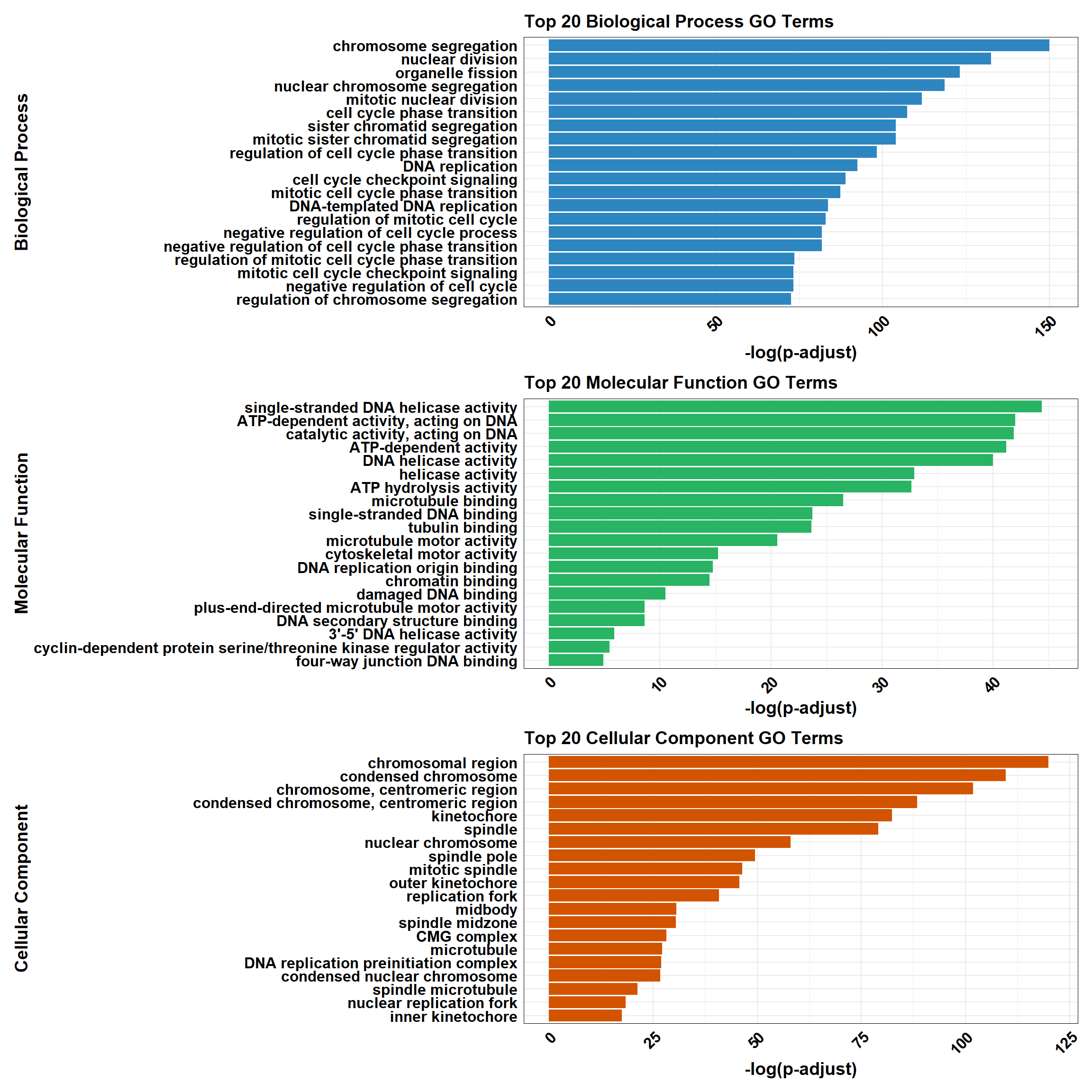
📌 CX vs VEH (0.5 and 24hr) GO Enrichment g:Profiler
# Load the gprofiler2 package
library(gprofiler2)
library(ggplot2)
library(dplyr)
library(patchwork)

# Perform GO enrichment analysis with gprofiler2
gost_results <- gost(
  query = DEG5,
  organism = "hsapiens",   # Human organism
  user_threshold = 0.05,   # Adjusted p-value cutoff
  correction_method = "fdr", # Multiple testing correction
  domain_scope = "custom", # Use custom background
  custom_bg = background,    # Background set of genes
  sources = c("GO:BP", "GO:MF", "GO:CC") # Analyze GO categories
)

# Check if enrichment results exist
if (is.null(gost_results$result) || nrow(gost_results$result) == 0) {
  # If no enriched terms, create a placeholder dataframe
  combined_results <- tibble(
    term_name = "No enriched terms",
    p.adjust = NA,
    source = "N/A",
    Category = "N/A"
  )
} else {
  # Convert results to a data frame
  gost_results_df <- gost_results$result

  # Add a column for adjusted p-value
  gost_results_df <- gost_results_df %>%
    rename(p.adjust = p_value)

  # Separate results for BP, MF, and CC
  BP_results <- gost_results_df %>%
    filter(source == "GO:BP") %>%
    mutate(Category = "Biological Process")

  MF_results <- gost_results_df %>%
    filter(source == "GO:MF") %>%
    mutate(Category = "Molecular Function")

  CC_results <- gost_results_df %>%
    filter(source == "GO:CC") %>%
    mutate(Category = "Cellular Component")

  # Select the top 20 terms by adjusted p-value for each category
  top_BP <- BP_results %>%
    arrange(p.adjust) %>%
    slice_head(n = 20)

  top_MF <- MF_results %>%
    arrange(p.adjust) %>%
    slice_head(n = 20)

  top_CC <- CC_results %>%
    arrange(p.adjust) %>%
    slice_head(n = 20)

  # Combine all categories
  combined_results <- bind_rows(top_BP, top_MF, top_CC)
}

# Ensure all columns are atomic types for CSV export
combined_results_clean <- combined_results %>%
  mutate(across(everything(), ~ if (is.list(.)) sapply(., toString) else .))

# Function for plotting top terms
plot_gprofiler_results <- function(data, title, color) {
  ggplot(data, aes(x = -log10(p.adjust), y = reorder(term_name, -log10(p.adjust)))) +
    geom_bar(stat = "identity", fill = color) +
    labs(
      x = "-log10(Adjusted p-value)",
      y = title,
      title = paste("Top 20", title, "GO Terms")
    ) +
    theme_minimal() +
    theme(
      axis.text.x = element_text(size = 12, face = "bold", colour = "black", angle = 45, hjust = 1),
      axis.text.y = element_text(size = 12, face = "bold", colour = "black"),
      axis.title.x = element_text(size = 14, face = "bold", colour = "black"),
      axis.title.y = element_text(size = 14, face = "bold", colour = "black"),
      plot.title = element_text(size = 14, face = "bold", colour = "black"),
      panel.border = element_rect(colour = "black", fill = NA, size = 0.3)
    )
}

# Check if there are enrichment terms to plot
if (nrow(combined_results) == 1 && combined_results$term_name == "No enriched terms") {
  message("No enriched GO terms found for the input gene set.")
} else {
  # Plot the top 20 terms for each category
  plot_BP <- plot_gprofiler_results(top_BP, "Biological Process", "#2E86C1")
  plot_MF <- plot_gprofiler_results(top_MF, "Molecular Function", "#28B463")
  plot_CC <- plot_gprofiler_results(top_CC, "Cellular Component", "#D35400")

  # Combine the plots using patchwork
  combined_plot <- plot_BP / plot_MF / plot_CC

  # Display the combined plot
  combined_plot
}
📌 CX vs VEH (0.5 and 24hr) Pathway Enrichment
# Load required libraries
library(clusterProfiler)
library(org.Hs.eg.db) # Required for enrichPathway
library(gprofiler2)
library(ggplot2)
library(dplyr)
library(patchwork)
library(ReactomePA)

# Function for ClusterProfiler Reactome & KEGG Analysis
process_clusterProfiler <- function(gene_set, background, category, color, y_title) {
  # Perform enrichment based on the selected category
  if (category == "Reactome") {
    enrichment <- enrichPathway(
      gene = gene_set,
      organism = "human",
      pvalueCutoff = 0.05,
      pAdjustMethod = "BH",
      universe = background
    )
  } else if (category == "KEGG") {
    enrichment <- enrichKEGG(
      gene = gene_set,
      organism = "hsa",
      pvalueCutoff = 0.05,
      pAdjustMethod = "BH",
      universe = background
    )
  }

  # Check if enrichment results exist
  if (is.null(enrichment) || nrow(as.data.frame(enrichment)) == 0) {
    message(paste("No significant enrichment found for", category, "in ClusterProfiler"))
    return(NULL)
  }

  # Convert results to tibble and process top 20 terms
  enrichment_tibble <- as_tibble(as.data.frame(enrichment)) %>%
    mutate(Category = category,
           neglog = -log10(p.adjust)) %>%  # Compute -log10(p.adjust)
    arrange(desc(neglog)) %>%
    slice_head(n = min(20, nrow(.)))  # Ensure safe slicing

  # Generate plot
  plot <- ggplot(enrichment_tibble, aes(x = neglog, y = reorder(Description, neglog))) +
    geom_bar(stat = "identity", fill = color) +
    labs(x = "-log10(Adjusted p-value)",
         y = y_title,
         title = paste("Enriched", category, "Pathways")) +
    theme_minimal() +
    theme(
      axis.text.x = element_text(size = 12, face = "bold", colour = "black", angle = 45, hjust = 1),
      axis.text.y = element_text(size = 12, face = "bold", colour = "black"),
      axis.title.x = element_text(size = 14, face = "bold", colour = "black"),
      axis.title.y = element_text(size = 14, face = "bold", colour = "black"),
      plot.title = element_text(size = 14, face = "bold", colour = "black")
    )

  return(plot)
}

# Function for gProfiler Reactome & KEGG Analysis
process_gprofiler <- function(gene_set, background, category, color, y_title) {
  # Perform enrichment using gprofiler2
  enrichment <- gost(
    query = gene_set,
    organism = "hsapiens",
    user_threshold = 0.05,
    correction_method = "fdr",
    domain_scope = "custom",
    custom_bg = background,
    sources = category # Either "REAC" or "KEGG"
  )

  # Check if enrichment results exist
  if (is.null(enrichment$result) || nrow(enrichment$result) == 0) {
    message(paste("No significant enrichment found for", category, "in gProfiler"))
    return(NULL)
  }

  # Convert results to tibble and process top 20 terms
  enrichment_tibble <- enrichment$result %>%
    as_tibble() %>%
    mutate(Category = category,
           neglog = -log10(p_value)) %>%  # Compute -log10(p-value)
    arrange(desc(neglog)) %>%
    slice_head(n = min(20, nrow(.)))  # Ensure safe slicing

  # Generate plot
  plot <- ggplot(enrichment_tibble, aes(x = neglog, y = reorder(term_name, neglog))) +
    geom_bar(stat = "identity", fill = color) +
    labs(x = "-log10(p-value)",
         y = y_title,
         title = paste("Enriched", category, "Pathways")) +
    theme_minimal() +
    theme(
      axis.text.x = element_text(size = 12, face = "bold", colour = "black", angle = 45, hjust = 1),
      axis.text.y = element_text(size = 12, face = "bold", colour = "black"),
      axis.title.x = element_text(size = 14, face = "bold", colour = "black"),
      axis.title.y = element_text(size = 14, face = "bold", colour = "black"),
      plot.title = element_text(size = 14, face = "bold", colour = "black")
    )

  return(plot)
}

# Perform analysis for Reactome and KEGG using ClusterProfiler
cluster_reactome <- process_clusterProfiler(
  gene_set = DEG5,
  background = background,
  category = "Reactome",
  color = "#2E86C1",
  y_title = "Reactome Pathways"
)

cluster_kegg <- process_clusterProfiler(
  gene_set = DEG5,
  background = background,
  category = "KEGG",
  color = "#28B463",
  y_title = "KEGG Pathways"
)

# Combine Reactome and KEGG for ClusterProfiler
if (!is.null(cluster_reactome) && !is.null(cluster_kegg)) {
  cluster_combined <- cluster_reactome / cluster_kegg
} else if (!is.null(cluster_reactome)) {
  cluster_combined <- cluster_reactome
} else if (!is.null(cluster_kegg)) {
  cluster_combined <- cluster_kegg
} else {
  cluster_combined <- NULL
}

# Perform analysis for Reactome and KEGG using GProfiler
gprofiler_reactome <- process_gprofiler(
  gene_set = DEG5,
  background = background,
  category = "REAC",  # Corrected category for Reactome in gProfiler
  color = "#D35400",
  y_title = "Reactome Pathways"
)

gprofiler_kegg <- process_gprofiler(
  gene_set = DEG5,
  background = background,
  category = "KEGG",
  color = "#F39C12",
  y_title = "KEGG Pathways"
)

# Combine Reactome and KEGG for GProfiler
if (!is.null(gprofiler_reactome) && !is.null(gprofiler_kegg)) {
  gprofiler_combined <- gprofiler_reactome / gprofiler_kegg
} else if (!is.null(gprofiler_reactome)) {
  gprofiler_combined <- gprofiler_reactome
} else if (!is.null(gprofiler_kegg)) {
  gprofiler_combined <- gprofiler_kegg
} else {
  gprofiler_combined <- NULL
}

# Display plots (if they are not NULL)
if (!is.null(cluster_combined)) print(cluster_combined)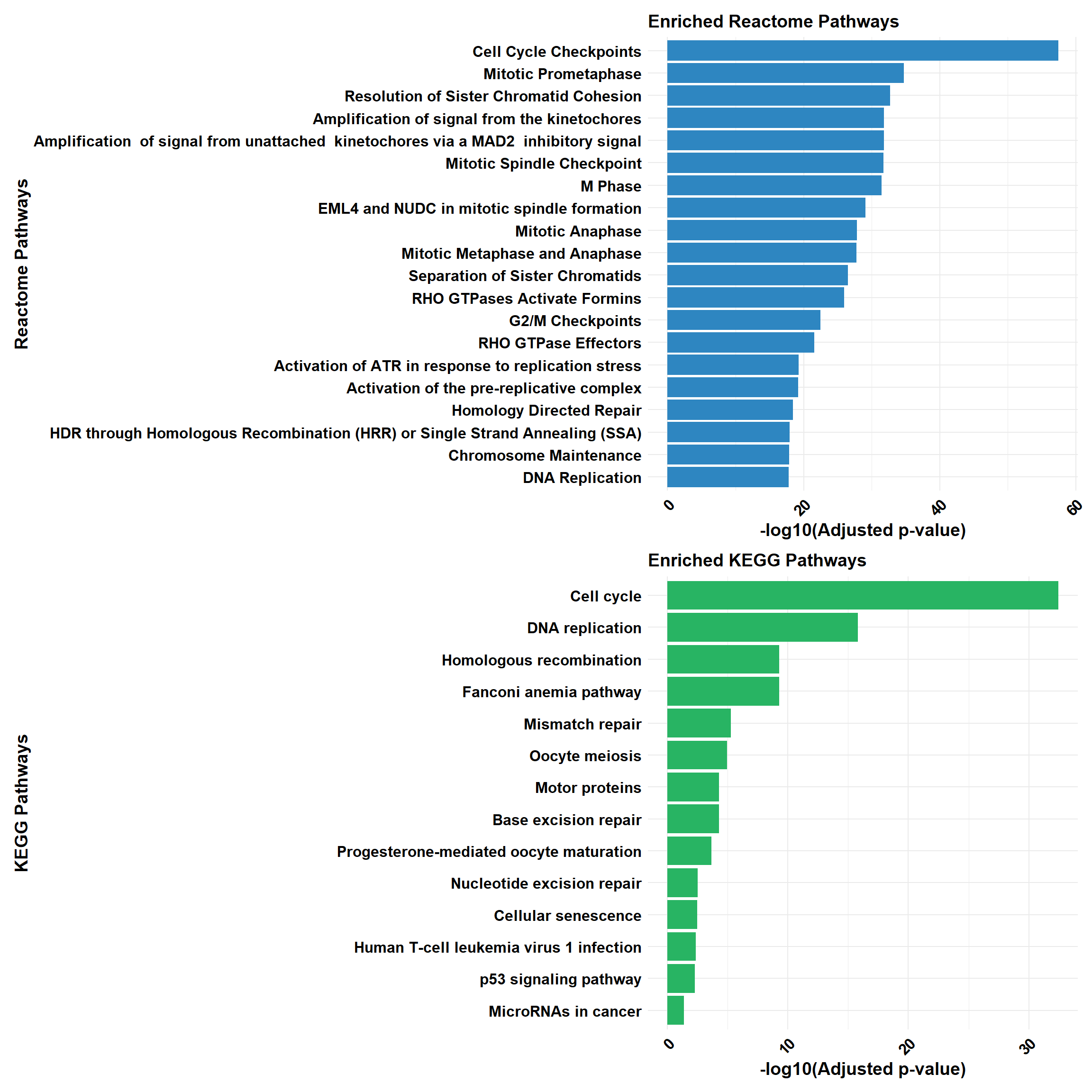
if (!is.null(gprofiler_combined)) print(gprofiler_combined)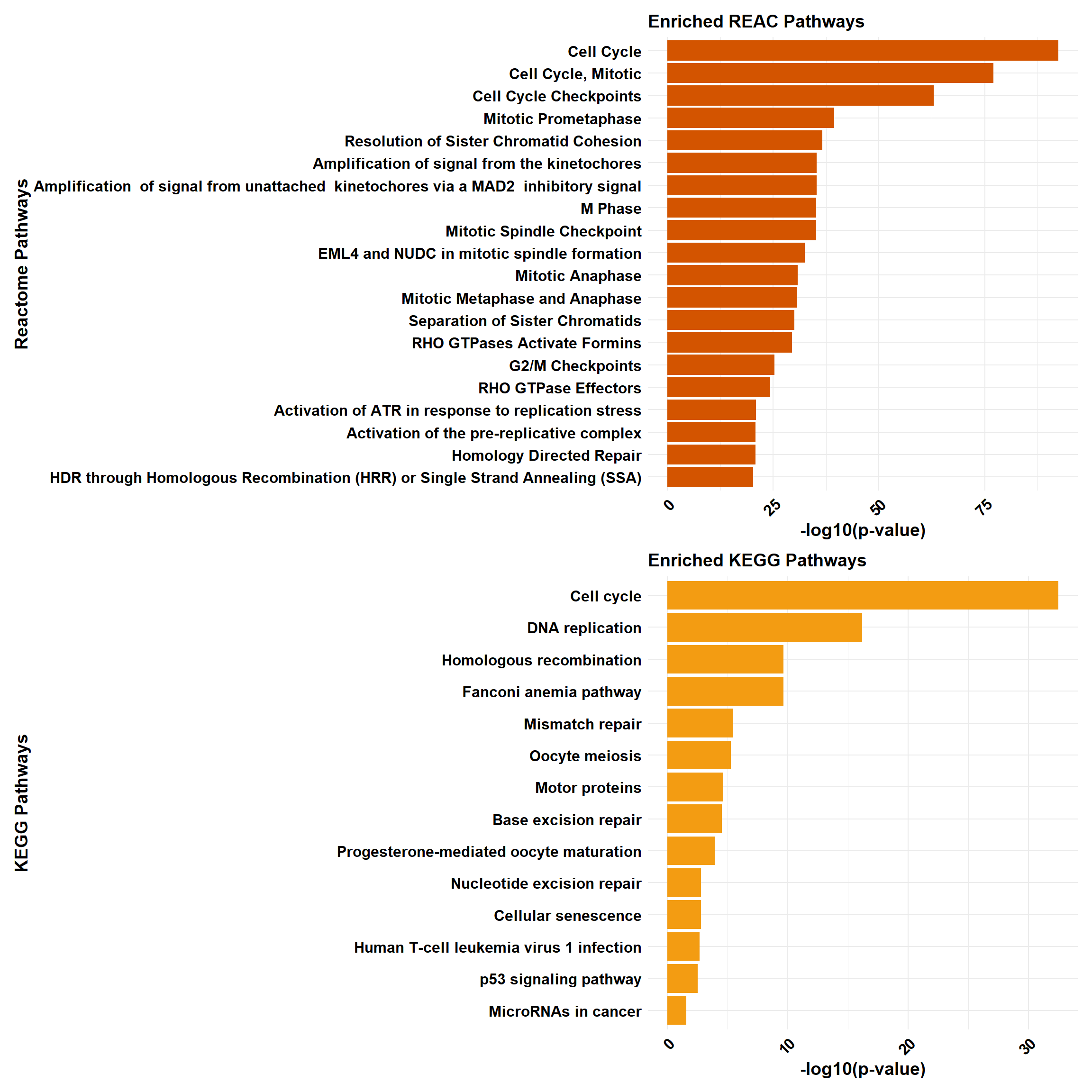
📌 CX vs VEH (0.5 and 48hr)
📌 CX vs VEH (0.5 and 48hr) GO Enrichment Clusterprofiler
# Perform GO enrichment analysis for BP, MF, and CC
go_enrichment_BP <- enrichGO(gene = DEG6,
                             OrgDb = org.Hs.eg.db,
                             keyType = "ENTREZID",
                             universe = background,
                             ont = "BP",
                             pvalueCutoff = 0.05)

go_enrichment_MF <- enrichGO(gene = DEG6,
                             OrgDb = org.Hs.eg.db,
                             keyType = "ENTREZID",
                             universe = background,
                             ont = "MF",
                             pvalueCutoff = 0.05)

go_enrichment_CC <- enrichGO(gene = DEG6,
                             OrgDb = org.Hs.eg.db,
                             keyType = "ENTREZID",
                             universe = background,
                             ont = "CC",
                             pvalueCutoff = 0.05)

# Convert each enrichment result to a tibble, add a category column, and select top 20 terms
process_enrichment_tibble <- function(enrichment, category) {
  if (is.null(enrichment) || nrow(as.data.frame(enrichment)) == 0) {
    return(tibble(Description = "No enriched terms", neglog = 0, Category = category))
  } else {
    enrichment %>%
      as_tibble() %>%
      mutate(Category = category,
             neglog = -log(p.adjust)) %>% # Add -log(p.adjust) column
      arrange(desc(neglog)) %>%          # Sort by -log(p.adjust)
      slice(1:20)                        # Select top 20 terms
  }
}

BP_Tibble <- process_enrichment_tibble(go_enrichment_BP, "Biological Process")
MF_Tibble <- process_enrichment_tibble(go_enrichment_MF, "Molecular Function")
CC_Tibble <- process_enrichment_tibble(go_enrichment_CC, "Cellular Component")

# Combine all tibbles
combined_GO_Tibble <- bind_rows(BP_Tibble, MF_Tibble, CC_Tibble)
# Function to generate enrichment plots
process_enrichment_plot <- function(tibble, title, color) {
  ggplot(data = tibble, aes(x = neglog, y = reorder(Description, neglog))) +
    geom_bar(stat = "identity", fill = color) +
    labs(x = "-log(p-adjust)",
         y = title,
         title = paste("Top 20", title, "GO Terms")) +
    theme_minimal() +
    theme(
      axis.text.x = element_text(size = 12, face = "bold", colour = "black", angle = 45, hjust = 1),
      axis.text.y = element_text(size = 12, face = "bold", colour = "black"),
      axis.title.x = element_text(size = 14, face = "bold", colour = "black"),
      axis.title.y = element_text(size = 14, face = "bold", colour = "black"),
      plot.title = element_text(size = 14, face = "bold", colour = "black"),
      panel.border = element_rect(colour = "black", fill = NA, size = 0.3)
    ) +
    xlim(c(0, max(tibble$neglog) + 1))
}

# Generate separate plots
plot_BP <- process_enrichment_plot(BP_Tibble, "Biological Process", "#2E86C1")
plot_MF <- process_enrichment_plot(MF_Tibble, "Molecular Function", "#28B463")
plot_CC <- process_enrichment_plot(CC_Tibble, "Cellular Component", "#D35400")

# Combine the plots using patchwork
combined_plot <- plot_BP / plot_MF / plot_CC

# Display the combined plot
combined_plot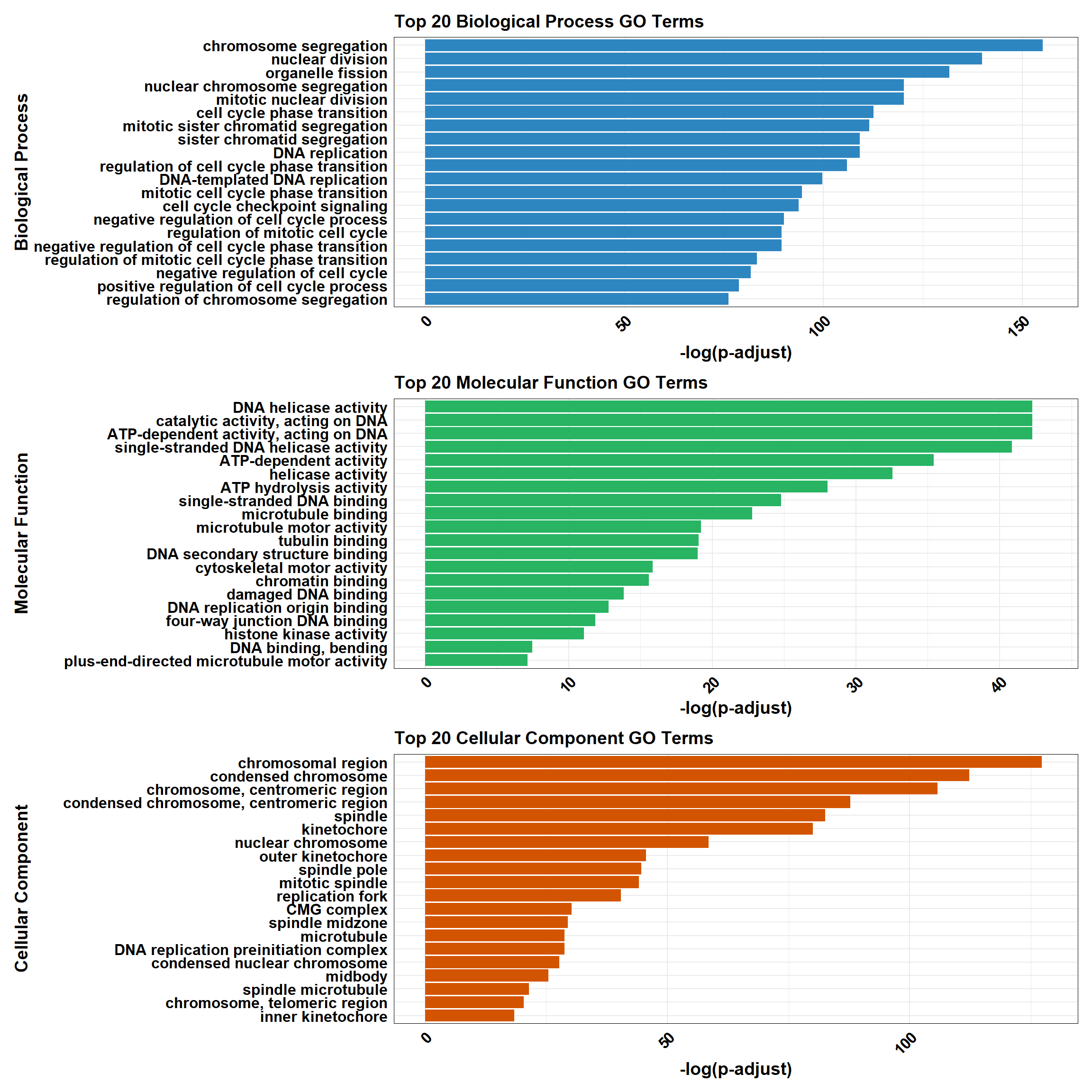
📌 CX vs VEH (0.5 and 48hr) GO Enrichment g:Profiler
# Load the gprofiler2 package
library(gprofiler2)
library(ggplot2)
library(dplyr)
library(patchwork)

# Perform GO enrichment analysis with gprofiler2
gost_results <- gost(
  query = DEG6,
  organism = "hsapiens",   # Human organism
  user_threshold = 0.05,   # Adjusted p-value cutoff
  correction_method = "fdr", # Multiple testing correction
  domain_scope = "custom", # Use custom background
  custom_bg = background,    # Background set of genes
  sources = c("GO:BP", "GO:MF", "GO:CC") # Analyze GO categories
)

# Check if enrichment results exist
if (is.null(gost_results$result) || nrow(gost_results$result) == 0) {
  # If no enriched terms, create a placeholder dataframe
  combined_results <- tibble(
    term_name = "No enriched terms",
    p.adjust = NA,
    source = "N/A",
    Category = "N/A"
  )
} else {
  # Convert results to a data frame
  gost_results_df <- gost_results$result

  # Add a column for adjusted p-value
  gost_results_df <- gost_results_df %>%
    rename(p.adjust = p_value)

  # Separate results for BP, MF, and CC
  BP_results <- gost_results_df %>%
    filter(source == "GO:BP") %>%
    mutate(Category = "Biological Process")

  MF_results <- gost_results_df %>%
    filter(source == "GO:MF") %>%
    mutate(Category = "Molecular Function")

  CC_results <- gost_results_df %>%
    filter(source == "GO:CC") %>%
    mutate(Category = "Cellular Component")

  # Select the top 20 terms by adjusted p-value for each category
  top_BP <- BP_results %>%
    arrange(p.adjust) %>%
    slice_head(n = 20)

  top_MF <- MF_results %>%
    arrange(p.adjust) %>%
    slice_head(n = 20)

  top_CC <- CC_results %>%
    arrange(p.adjust) %>%
    slice_head(n = 20)

  # Combine all categories
  combined_results <- bind_rows(top_BP, top_MF, top_CC)
}

# Ensure all columns are atomic types for CSV export
combined_results_clean <- combined_results %>%
  mutate(across(everything(), ~ if (is.list(.)) sapply(., toString) else .))

# Function for plotting top terms
plot_gprofiler_results <- function(data, title, color) {
  ggplot(data, aes(x = -log10(p.adjust), y = reorder(term_name, -log10(p.adjust)))) +
    geom_bar(stat = "identity", fill = color) +
    labs(
      x = "-log10(Adjusted p-value)",
      y = title,
      title = paste("Top 20", title, "GO Terms")
    ) +
    theme_minimal() +
    theme(
      axis.text.x = element_text(size = 12, face = "bold", colour = "black", angle = 45, hjust = 1),
      axis.text.y = element_text(size = 12, face = "bold", colour = "black"),
      axis.title.x = element_text(size = 14, face = "bold", colour = "black"),
      axis.title.y = element_text(size = 14, face = "bold", colour = "black"),
      plot.title = element_text(size = 14, face = "bold", colour = "black"),
      panel.border = element_rect(colour = "black", fill = NA, size = 0.3)
    )
}

# Check if there are enrichment terms to plot
if (nrow(combined_results) == 1 && combined_results$term_name == "No enriched terms") {
  message("No enriched GO terms found for the input gene set.")
} else {
  # Plot the top 20 terms for each category
  plot_BP <- plot_gprofiler_results(top_BP, "Biological Process", "#2E86C1")
  plot_MF <- plot_gprofiler_results(top_MF, "Molecular Function", "#28B463")
  plot_CC <- plot_gprofiler_results(top_CC, "Cellular Component", "#D35400")

  # Combine the plots using patchwork
  combined_plot <- plot_BP / plot_MF / plot_CC

  # Display the combined plot
  combined_plot
}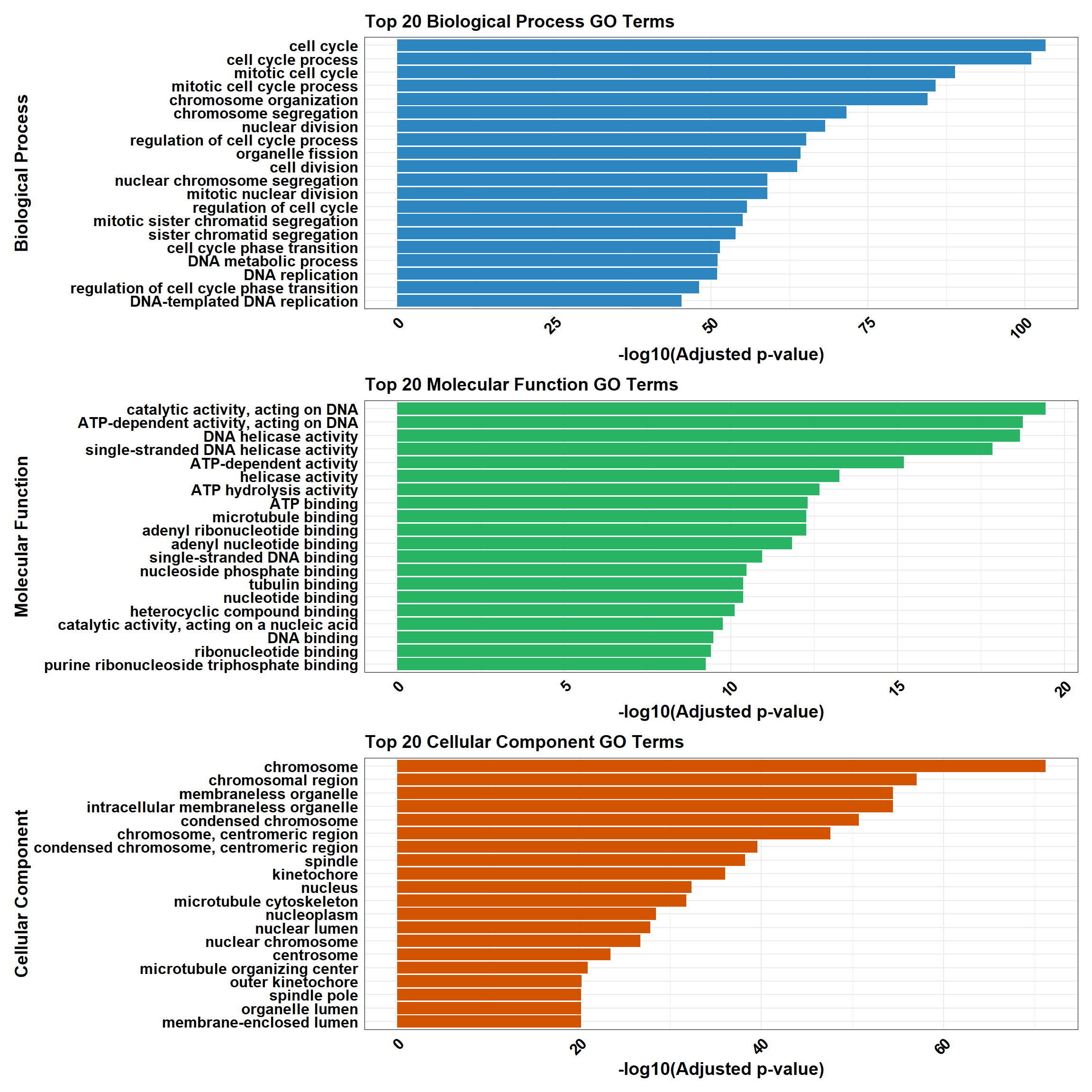
📌 CX vs VEH (0.5 and 48hr) Pathway Enrichment
# Load required libraries
library(clusterProfiler)
library(org.Hs.eg.db) # Required for enrichPathway
library(gprofiler2)
library(ggplot2)
library(dplyr)
library(patchwork)
library(ReactomePA)

# Function for ClusterProfiler Reactome & KEGG Analysis
process_clusterProfiler <- function(gene_set, background, category, color, y_title) {
  # Perform enrichment based on the selected category
  if (category == "Reactome") {
    enrichment <- enrichPathway(
      gene = gene_set,
      organism = "human",
      pvalueCutoff = 0.05,
      pAdjustMethod = "BH",
      universe = background
    )
  } else if (category == "KEGG") {
    enrichment <- enrichKEGG(
      gene = gene_set,
      organism = "hsa",
      pvalueCutoff = 0.05,
      pAdjustMethod = "BH",
      universe = background
    )
  }

  # Check if enrichment results exist
  if (is.null(enrichment) || nrow(as.data.frame(enrichment)) == 0) {
    message(paste("No significant enrichment found for", category, "in ClusterProfiler"))
    return(NULL)
  }

  # Convert results to tibble and process top 20 terms
  enrichment_tibble <- as_tibble(as.data.frame(enrichment)) %>%
    mutate(Category = category,
           neglog = -log10(p.adjust)) %>%  # Compute -log10(p.adjust)
    arrange(desc(neglog)) %>%
    slice_head(n = min(20, nrow(.)))  # Ensure safe slicing

  # Generate plot
  plot <- ggplot(enrichment_tibble, aes(x = neglog, y = reorder(Description, neglog))) +
    geom_bar(stat = "identity", fill = color) +
    labs(x = "-log10(Adjusted p-value)",
         y = y_title,
         title = paste("Enriched", category, "Pathways")) +
    theme_minimal() +
    theme(
      axis.text.x = element_text(size = 12, face = "bold", colour = "black", angle = 45, hjust = 1),
      axis.text.y = element_text(size = 12, face = "bold", colour = "black"),
      axis.title.x = element_text(size = 14, face = "bold", colour = "black"),
      axis.title.y = element_text(size = 14, face = "bold", colour = "black"),
      plot.title = element_text(size = 14, face = "bold", colour = "black")
    )

  return(plot)
}

# Function for gProfiler Reactome & KEGG Analysis
process_gprofiler <- function(gene_set, background, category, color, y_title) {
  # Perform enrichment using gprofiler2
  enrichment <- gost(
    query = gene_set,
    organism = "hsapiens",
    user_threshold = 0.05,
    correction_method = "fdr",
    domain_scope = "custom",
    custom_bg = background,
    sources = category # Either "REAC" or "KEGG"
  )

  # Check if enrichment results exist
  if (is.null(enrichment$result) || nrow(enrichment$result) == 0) {
    message(paste("No significant enrichment found for", category, "in gProfiler"))
    return(NULL)
  }

  # Convert results to tibble and process top 20 terms
  enrichment_tibble <- enrichment$result %>%
    as_tibble() %>%
    mutate(Category = category,
           neglog = -log10(p_value)) %>%  # Compute -log10(p-value)
    arrange(desc(neglog)) %>%
    slice_head(n = min(20, nrow(.)))  # Ensure safe slicing

  # Generate plot
  plot <- ggplot(enrichment_tibble, aes(x = neglog, y = reorder(term_name, neglog))) +
    geom_bar(stat = "identity", fill = color) +
    labs(x = "-log10(p-value)",
         y = y_title,
         title = paste("Enriched", category, "Pathways")) +
    theme_minimal() +
    theme(
      axis.text.x = element_text(size = 12, face = "bold", colour = "black", angle = 45, hjust = 1),
      axis.text.y = element_text(size = 12, face = "bold", colour = "black"),
      axis.title.x = element_text(size = 14, face = "bold", colour = "black"),
      axis.title.y = element_text(size = 14, face = "bold", colour = "black"),
      plot.title = element_text(size = 14, face = "bold", colour = "black")
    )

  return(plot)
}

# Perform analysis for Reactome and KEGG using ClusterProfiler
cluster_reactome <- process_clusterProfiler(
  gene_set = DEG6,
  background = background,
  category = "Reactome",
  color = "#2E86C1",
  y_title = "Reactome Pathways"
)

cluster_kegg <- process_clusterProfiler(
  gene_set = DEG6,
  background = background,
  category = "KEGG",
  color = "#28B463",
  y_title = "KEGG Pathways"
)

# Combine Reactome and KEGG for ClusterProfiler
if (!is.null(cluster_reactome) && !is.null(cluster_kegg)) {
  cluster_combined <- cluster_reactome / cluster_kegg
} else if (!is.null(cluster_reactome)) {
  cluster_combined <- cluster_reactome
} else if (!is.null(cluster_kegg)) {
  cluster_combined <- cluster_kegg
} else {
  cluster_combined <- NULL
}

# Perform analysis for Reactome and KEGG using GProfiler
gprofiler_reactome <- process_gprofiler(
  gene_set = DEG6,
  background = background,
  category = "REAC",  # Corrected category for Reactome in gProfiler
  color = "#D35400",
  y_title = "Reactome Pathways"
)

gprofiler_kegg <- process_gprofiler(
  gene_set = DEG6,
  background = background,
  category = "KEGG",
  color = "#F39C12",
  y_title = "KEGG Pathways"
)

# Combine Reactome and KEGG for GProfiler
if (!is.null(gprofiler_reactome) && !is.null(gprofiler_kegg)) {
  gprofiler_combined <- gprofiler_reactome / gprofiler_kegg
} else if (!is.null(gprofiler_reactome)) {
  gprofiler_combined <- gprofiler_reactome
} else if (!is.null(gprofiler_kegg)) {
  gprofiler_combined <- gprofiler_kegg
} else {
  gprofiler_combined <- NULL
}

# Display plots (if they are not NULL)
if (!is.null(cluster_combined)) print(cluster_combined)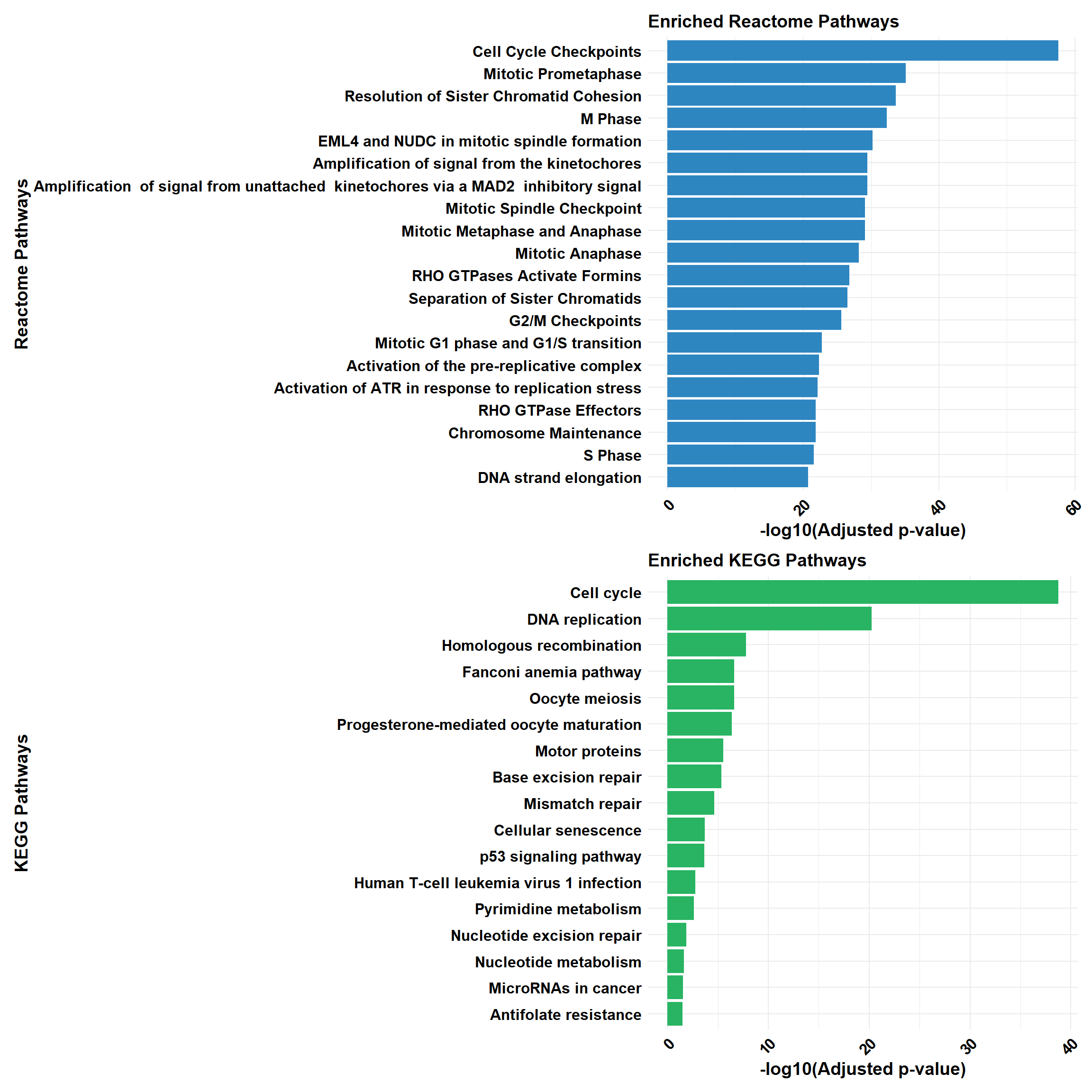
if (!is.null(gprofiler_combined)) print(gprofiler_combined)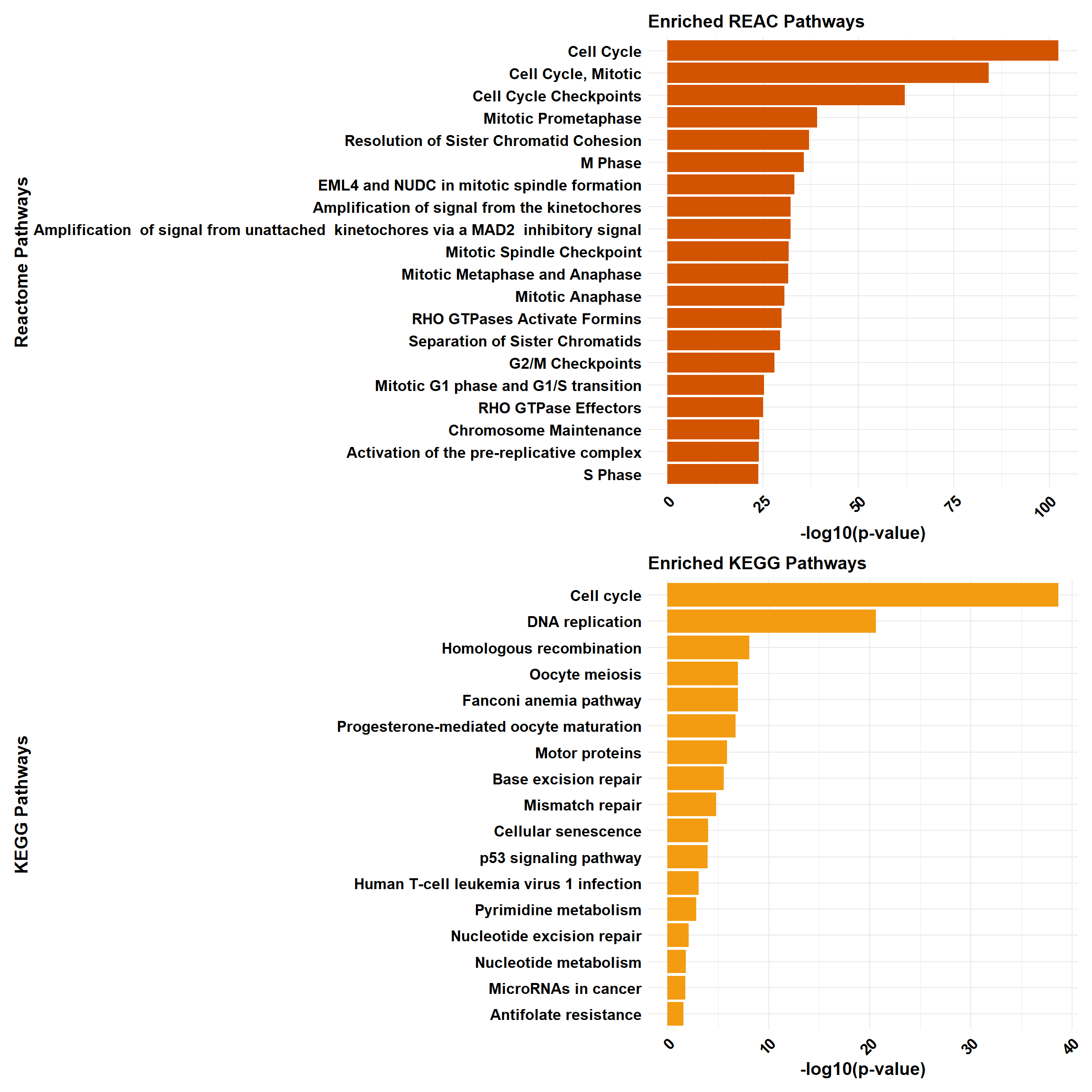
📌 DOX vs VEH (0.1 and 3hr)
📌 DOX vs VEH (0.1 and 3hr) GO Enrichment Clusterprofiler
# Perform GO enrichment analysis for BP, MF, and CC
go_enrichment_BP <- enrichGO(gene = DEG7,
                             OrgDb = org.Hs.eg.db,
                             keyType = "ENTREZID",
                             universe = background,
                             ont = "BP",
                             pvalueCutoff = 0.05)

go_enrichment_MF <- enrichGO(gene = DEG7,
                             OrgDb = org.Hs.eg.db,
                             keyType = "ENTREZID",
                             universe = background,
                             ont = "MF",
                             pvalueCutoff = 0.05)

go_enrichment_CC <- enrichGO(gene = DEG7,
                             OrgDb = org.Hs.eg.db,
                             keyType = "ENTREZID",
                             universe = background,
                             ont = "CC",
                             pvalueCutoff = 0.05)

# Convert each enrichment result to a tibble, add a category column, and select top 20 terms
process_enrichment_tibble <- function(enrichment, category) {
  if (is.null(enrichment) || nrow(as.data.frame(enrichment)) == 0) {
    return(tibble(Description = "No enriched terms", neglog = 0, Category = category))
  } else {
    enrichment %>%
      as_tibble() %>%
      mutate(Category = category,
             neglog = -log(p.adjust)) %>% # Add -log(p.adjust) column
      arrange(desc(neglog)) %>%          # Sort by -log(p.adjust)
      slice(1:20)                        # Select top 20 terms
  }
}

BP_Tibble <- process_enrichment_tibble(go_enrichment_BP, "Biological Process")
MF_Tibble <- process_enrichment_tibble(go_enrichment_MF, "Molecular Function")
CC_Tibble <- process_enrichment_tibble(go_enrichment_CC, "Cellular Component")

# Combine all tibbles
combined_GO_Tibble <- bind_rows(BP_Tibble, MF_Tibble, CC_Tibble)
# Function to generate enrichment plots
process_enrichment_plot <- function(tibble, title, color) {
  ggplot(data = tibble, aes(x = neglog, y = reorder(Description, neglog))) +
    geom_bar(stat = "identity", fill = color) +
    labs(x = "-log(p-adjust)",
         y = title,
         title = paste("Top 20", title, "GO Terms")) +
    theme_minimal() +
    theme(
      axis.text.x = element_text(size = 12, face = "bold", colour = "black", angle = 45, hjust = 1),
      axis.text.y = element_text(size = 12, face = "bold", colour = "black"),
      axis.title.x = element_text(size = 14, face = "bold", colour = "black"),
      axis.title.y = element_text(size = 14, face = "bold", colour = "black"),
      plot.title = element_text(size = 14, face = "bold", colour = "black"),
      panel.border = element_rect(colour = "black", fill = NA, size = 0.3)
    ) +
    xlim(c(0, max(tibble$neglog) + 1))
}

# Generate separate plots
plot_BP <- process_enrichment_plot(BP_Tibble, "Biological Process", "#2E86C1")
plot_MF <- process_enrichment_plot(MF_Tibble, "Molecular Function", "#28B463")
plot_CC <- process_enrichment_plot(CC_Tibble, "Cellular Component", "#D35400")

# Combine the plots using patchwork
combined_plot <- plot_BP / plot_MF / plot_CC

# Display the combined plot
combined_plot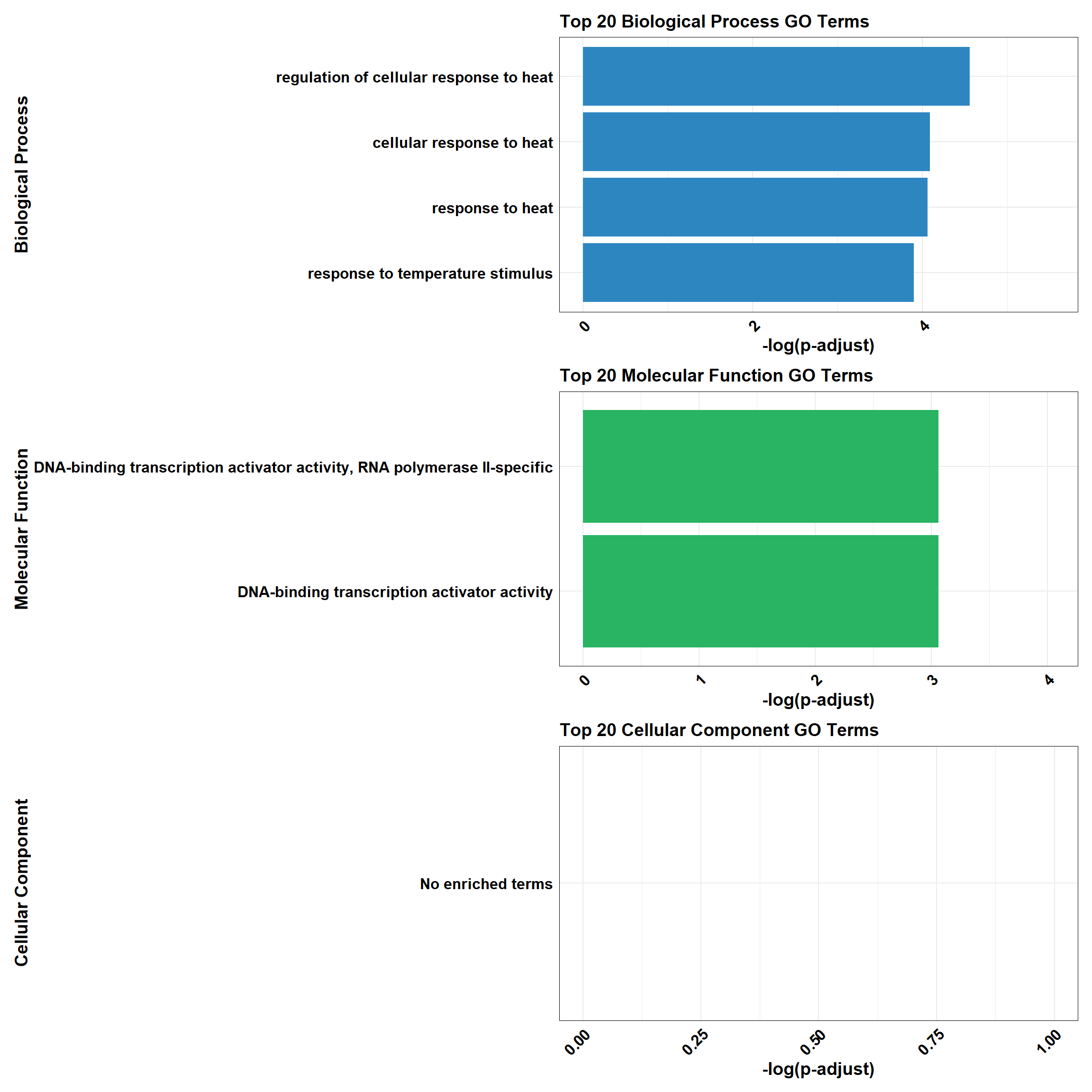
📌 DOX vs VEH (0.1 and 3hr) GO Enrichment g:Profiler
# Load the gprofiler2 package
library(gprofiler2)
library(ggplot2)
library(dplyr)
library(patchwork)

# Perform GO enrichment analysis with gprofiler2
gost_results <- gost(
  query = DEG7,
  organism = "hsapiens",   # Human organism
  user_threshold = 0.05,   # Adjusted p-value cutoff
  correction_method = "fdr", # Multiple testing correction
  domain_scope = "custom", # Use custom background
  custom_bg = background,    # Background set of genes
  sources = c("GO:BP", "GO:MF", "GO:CC") # Analyze GO categories
)

# Check if enrichment results exist
if (is.null(gost_results$result) || nrow(gost_results$result) == 0) {
  # If no enriched terms, create a placeholder dataframe
  combined_results <- tibble(
    term_name = "No enriched terms",
    p.adjust = NA,
    source = "N/A",
    Category = "N/A"
  )
} else {
  # Convert results to a data frame
  gost_results_df <- gost_results$result

  # Add a column for adjusted p-value
  gost_results_df <- gost_results_df %>%
    rename(p.adjust = p_value)

  # Separate results for BP, MF, and CC
  BP_results <- gost_results_df %>%
    filter(source == "GO:BP") %>%
    mutate(Category = "Biological Process")

  MF_results <- gost_results_df %>%
    filter(source == "GO:MF") %>%
    mutate(Category = "Molecular Function")

  CC_results <- gost_results_df %>%
    filter(source == "GO:CC") %>%
    mutate(Category = "Cellular Component")

  # Select the top 20 terms by adjusted p-value for each category
  top_BP <- BP_results %>%
    arrange(p.adjust) %>%
    slice_head(n = 20)

  top_MF <- MF_results %>%
    arrange(p.adjust) %>%
    slice_head(n = 20)

  top_CC <- CC_results %>%
    arrange(p.adjust) %>%
    slice_head(n = 20)

  # Combine all categories
  combined_results <- bind_rows(top_BP, top_MF, top_CC)
}

# Ensure all columns are atomic types for CSV export
combined_results_clean <- combined_results %>%
  mutate(across(everything(), ~ if (is.list(.)) sapply(., toString) else .))

# Function for plotting top terms
plot_gprofiler_results <- function(data, title, color) {
  ggplot(data, aes(x = -log10(p.adjust), y = reorder(term_name, -log10(p.adjust)))) +
    geom_bar(stat = "identity", fill = color) +
    labs(
      x = "-log10(Adjusted p-value)",
      y = title,
      title = paste("Top 20", title, "GO Terms")
    ) +
    theme_minimal() +
    theme(
      axis.text.x = element_text(size = 12, face = "bold", colour = "black", angle = 45, hjust = 1),
      axis.text.y = element_text(size = 12, face = "bold", colour = "black"),
      axis.title.x = element_text(size = 14, face = "bold", colour = "black"),
      axis.title.y = element_text(size = 14, face = "bold", colour = "black"),
      plot.title = element_text(size = 14, face = "bold", colour = "black"),
      panel.border = element_rect(colour = "black", fill = NA, size = 0.3)
    )
}

# Check if there are enrichment terms to plot
if (nrow(combined_results) == 1 && combined_results$term_name == "No enriched terms") {
  message("No enriched GO terms found for the input gene set.")
} else {
  # Plot the top 20 terms for each category
  plot_BP <- plot_gprofiler_results(top_BP, "Biological Process", "#2E86C1")
  plot_MF <- plot_gprofiler_results(top_MF, "Molecular Function", "#28B463")
  plot_CC <- plot_gprofiler_results(top_CC, "Cellular Component", "#D35400")

  # Combine the plots using patchwork
  combined_plot <- plot_BP / plot_MF / plot_CC

  # Display the combined plot
  combined_plot
}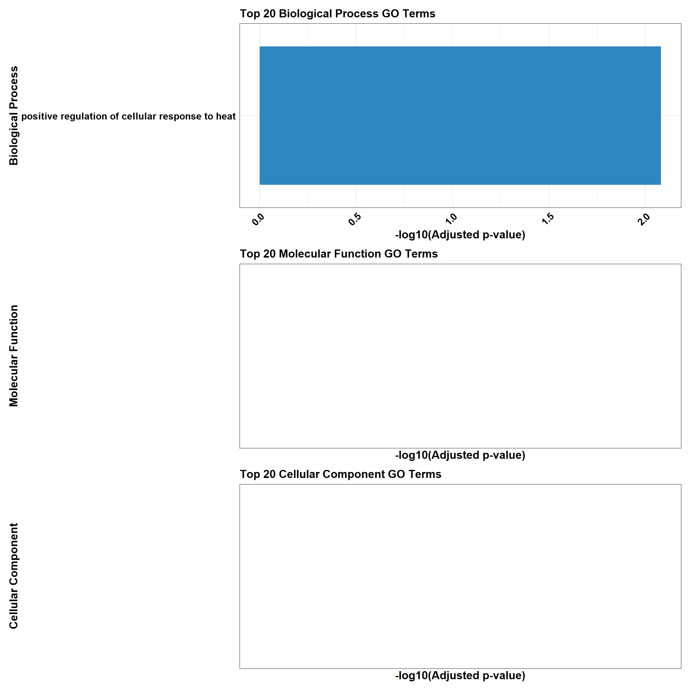
📌 DOX vs VEH (0.1 and 3hr) Pathway Enrichment
# Load required libraries
library(clusterProfiler)
library(org.Hs.eg.db) # Required for enrichPathway
library(gprofiler2)
library(ggplot2)
library(dplyr)
library(patchwork)
library(ReactomePA)

# Function for ClusterProfiler Reactome & KEGG Analysis
process_clusterProfiler <- function(gene_set, background, category, color, y_title) {
  # Perform enrichment based on the selected category
  if (category == "Reactome") {
    enrichment <- enrichPathway(
      gene = gene_set,
      organism = "human",
      pvalueCutoff = 0.05,
      pAdjustMethod = "BH",
      universe = background
    )
  } else if (category == "KEGG") {
    enrichment <- enrichKEGG(
      gene = gene_set,
      organism = "hsa",
      pvalueCutoff = 0.05,
      pAdjustMethod = "BH",
      universe = background
    )
  }

  # Check if enrichment results exist
  if (is.null(enrichment) || nrow(as.data.frame(enrichment)) == 0) {
    message(paste("No significant enrichment found for", category, "in ClusterProfiler"))
    return(NULL)
  }

  # Convert results to tibble and process top 20 terms
  enrichment_tibble <- as_tibble(as.data.frame(enrichment)) %>%
    mutate(Category = category,
           neglog = -log10(p.adjust)) %>%  # Compute -log10(p.adjust)
    arrange(desc(neglog)) %>%
    slice_head(n = min(20, nrow(.)))  # Ensure safe slicing

  # Generate plot
  plot <- ggplot(enrichment_tibble, aes(x = neglog, y = reorder(Description, neglog))) +
    geom_bar(stat = "identity", fill = color) +
    labs(x = "-log10(Adjusted p-value)",
         y = y_title,
         title = paste("Enriched", category, "Pathways")) +
    theme_minimal() +
    theme(
      axis.text.x = element_text(size = 12, face = "bold", colour = "black", angle = 45, hjust = 1),
      axis.text.y = element_text(size = 12, face = "bold", colour = "black"),
      axis.title.x = element_text(size = 14, face = "bold", colour = "black"),
      axis.title.y = element_text(size = 14, face = "bold", colour = "black"),
      plot.title = element_text(size = 14, face = "bold", colour = "black")
    )

  return(plot)
}

# Function for gProfiler Reactome & KEGG Analysis
process_gprofiler <- function(gene_set, background, category, color, y_title) {
  # Perform enrichment using gprofiler2
  enrichment <- gost(
    query = gene_set,
    organism = "hsapiens",
    user_threshold = 0.05,
    correction_method = "fdr",
    domain_scope = "custom",
    custom_bg = background,
    sources = category # Either "REAC" or "KEGG"
  )

  # Check if enrichment results exist
  if (is.null(enrichment$result) || nrow(enrichment$result) == 0) {
    message(paste("No significant enrichment found for", category, "in gProfiler"))
    return(NULL)
  }

  # Convert results to tibble and process top 20 terms
  enrichment_tibble <- enrichment$result %>%
    as_tibble() %>%
    mutate(Category = category,
           neglog = -log10(p_value)) %>%  # Compute -log10(p-value)
    arrange(desc(neglog)) %>%
    slice_head(n = min(20, nrow(.)))  # Ensure safe slicing

  # Generate plot
  plot <- ggplot(enrichment_tibble, aes(x = neglog, y = reorder(term_name, neglog))) +
    geom_bar(stat = "identity", fill = color) +
    labs(x = "-log10(p-value)",
         y = y_title,
         title = paste("Enriched", category, "Pathways")) +
    theme_minimal() +
    theme(
      axis.text.x = element_text(size = 12, face = "bold", colour = "black", angle = 45, hjust = 1),
      axis.text.y = element_text(size = 12, face = "bold", colour = "black"),
      axis.title.x = element_text(size = 14, face = "bold", colour = "black"),
      axis.title.y = element_text(size = 14, face = "bold", colour = "black"),
      plot.title = element_text(size = 14, face = "bold", colour = "black")
    )

  return(plot)
}

# Perform analysis for Reactome and KEGG using ClusterProfiler
cluster_reactome <- process_clusterProfiler(
  gene_set = DEG7,
  background = background,
  category = "Reactome",
  color = "#2E86C1",
  y_title = "Reactome Pathways"
)

cluster_kegg <- process_clusterProfiler(
  gene_set = DEG7,
  background = background,
  category = "KEGG",
  color = "#28B463",
  y_title = "KEGG Pathways"
)

# Combine Reactome and KEGG for ClusterProfiler
if (!is.null(cluster_reactome) && !is.null(cluster_kegg)) {
  cluster_combined <- cluster_reactome / cluster_kegg
} else if (!is.null(cluster_reactome)) {
  cluster_combined <- cluster_reactome
} else if (!is.null(cluster_kegg)) {
  cluster_combined <- cluster_kegg
} else {
  cluster_combined <- NULL
}

# Perform analysis for Reactome and KEGG using GProfiler
gprofiler_reactome <- process_gprofiler(
  gene_set = DEG7,
  background = background,
  category = "REAC",  # Corrected category for Reactome in gProfiler
  color = "#D35400",
  y_title = "Reactome Pathways"
)

gprofiler_kegg <- process_gprofiler(
  gene_set = DEG7,
  background = background,
  category = "KEGG",
  color = "#F39C12",
  y_title = "KEGG Pathways"
)

# Combine Reactome and KEGG for GProfiler
if (!is.null(gprofiler_reactome) && !is.null(gprofiler_kegg)) {
  gprofiler_combined <- gprofiler_reactome / gprofiler_kegg
} else if (!is.null(gprofiler_reactome)) {
  gprofiler_combined <- gprofiler_reactome
} else if (!is.null(gprofiler_kegg)) {
  gprofiler_combined <- gprofiler_kegg
} else {
  gprofiler_combined <- NULL
}

# Display plots (if they are not NULL)
if (!is.null(cluster_combined)) print(cluster_combined)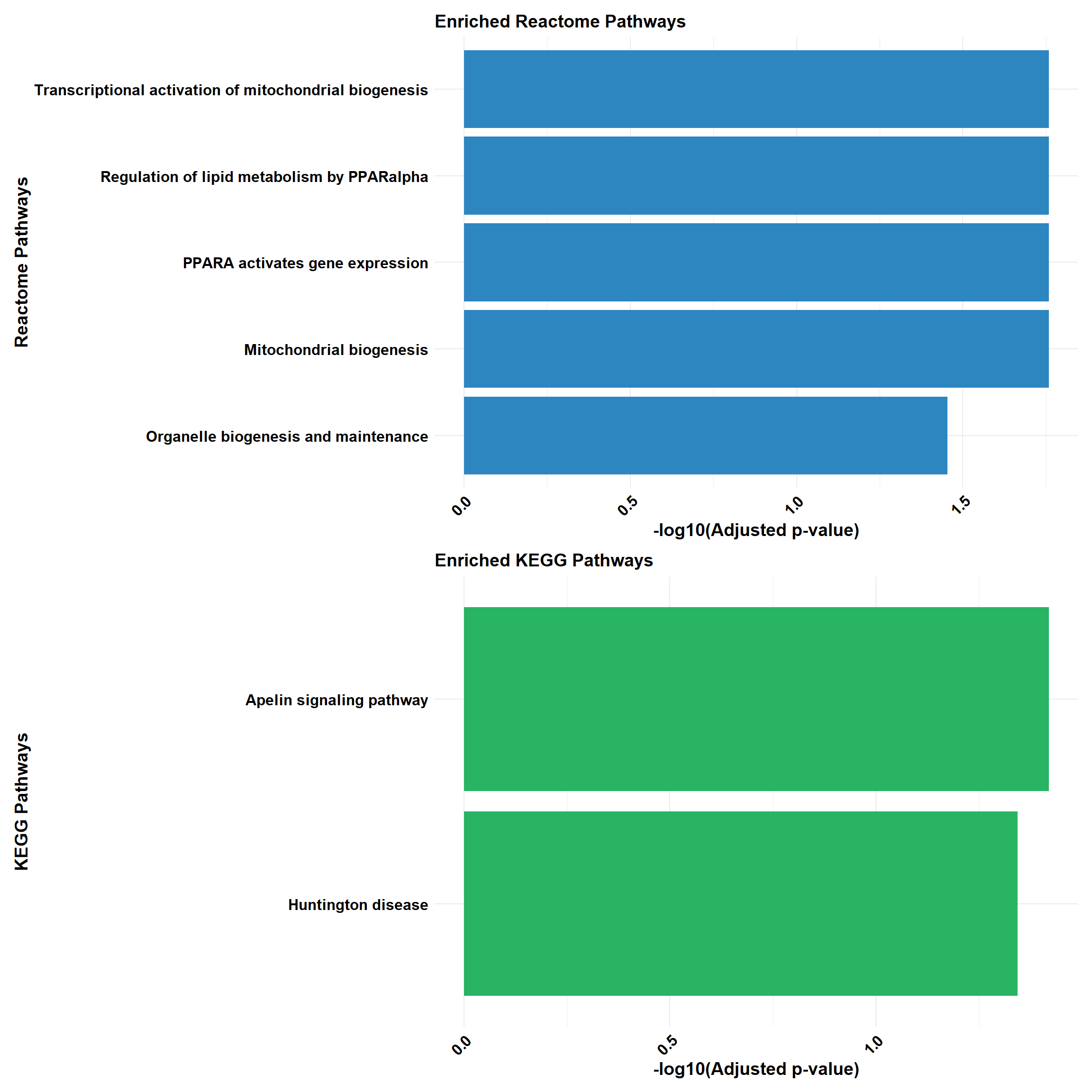
if (!is.null(gprofiler_combined)) print(gprofiler_combined)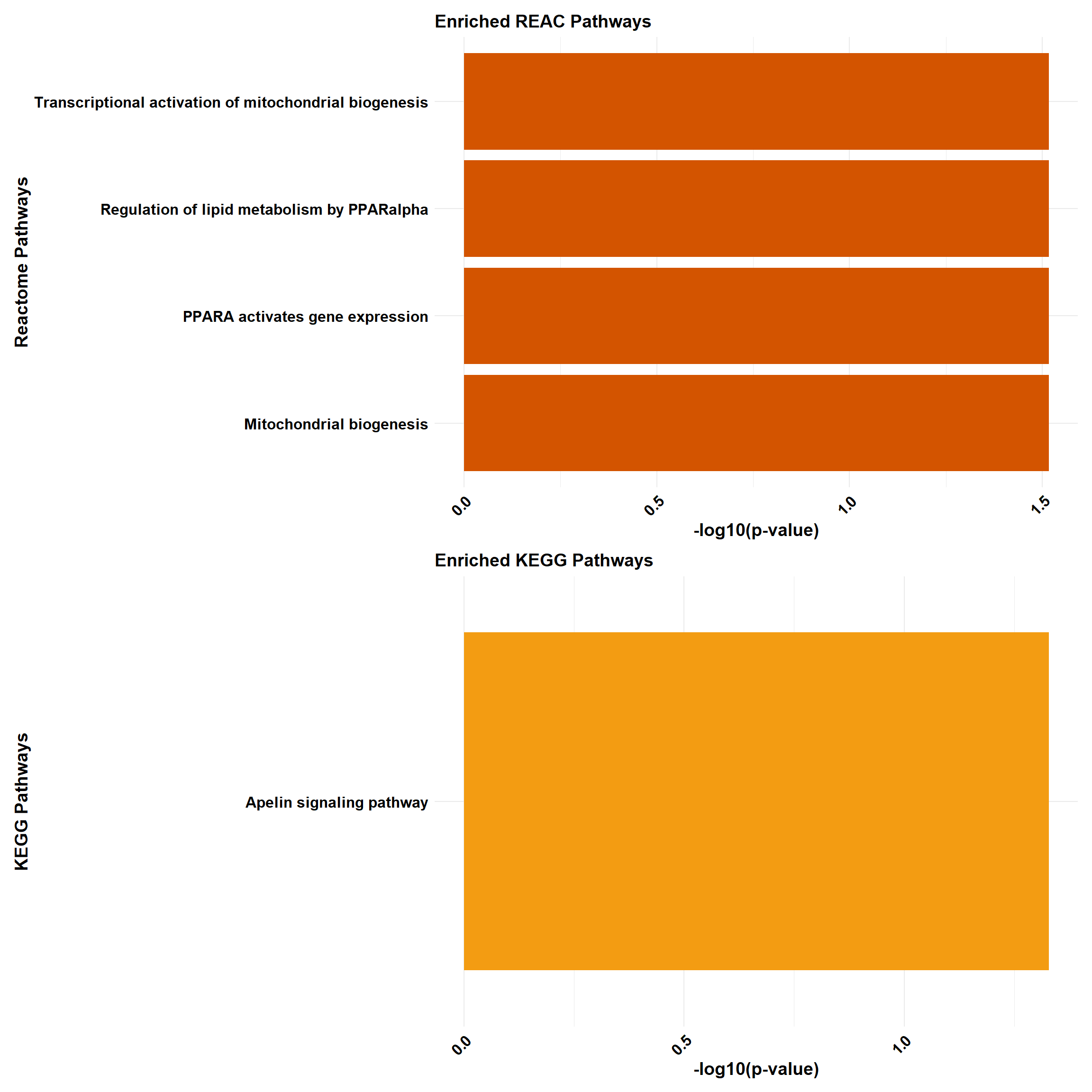
📌 DOX vs VEH (0.1 and 24hr)
📌 DOX vs VEH (0.1 and 24hr) GO Enrichment Clusterprofiler
# Perform GO enrichment analysis for BP, MF, and CC
go_enrichment_BP <- enrichGO(gene = DEG8,
                             OrgDb = org.Hs.eg.db,
                             keyType = "ENTREZID",
                             universe = background,
                             ont = "BP",
                             pvalueCutoff = 0.05)

go_enrichment_MF <- enrichGO(gene = DEG8,
                             OrgDb = org.Hs.eg.db,
                             keyType = "ENTREZID",
                             universe = background,
                             ont = "MF",
                             pvalueCutoff = 0.05)

go_enrichment_CC <- enrichGO(gene = DEG8,
                             OrgDb = org.Hs.eg.db,
                             keyType = "ENTREZID",
                             universe = background,
                             ont = "CC",
                             pvalueCutoff = 0.05)

# Convert each enrichment result to a tibble, add a category column, and select top 20 terms
process_enrichment_tibble <- function(enrichment, category) {
  if (is.null(enrichment) || nrow(as.data.frame(enrichment)) == 0) {
    return(tibble(Description = "No enriched terms", neglog = 0, Category = category))
  } else {
    enrichment %>%
      as_tibble() %>%
      mutate(Category = category,
             neglog = -log(p.adjust)) %>% # Add -log(p.adjust) column
      arrange(desc(neglog)) %>%          # Sort by -log(p.adjust)
      slice(1:20)                        # Select top 20 terms
  }
}

BP_Tibble <- process_enrichment_tibble(go_enrichment_BP, "Biological Process")
MF_Tibble <- process_enrichment_tibble(go_enrichment_MF, "Molecular Function")
CC_Tibble <- process_enrichment_tibble(go_enrichment_CC, "Cellular Component")

# Combine all tibbles
combined_GO_Tibble <- bind_rows(BP_Tibble, MF_Tibble, CC_Tibble)
# Function to generate enrichment plots
process_enrichment_plot <- function(tibble, title, color) {
  ggplot(data = tibble, aes(x = neglog, y = reorder(Description, neglog))) +
    geom_bar(stat = "identity", fill = color) +
    labs(x = "-log(p-adjust)",
         y = title,
         title = paste("Top 20", title, "GO Terms")) +
    theme_minimal() +
    theme(
      axis.text.x = element_text(size = 12, face = "bold", colour = "black", angle = 45, hjust = 1),
      axis.text.y = element_text(size = 12, face = "bold", colour = "black"),
      axis.title.x = element_text(size = 14, face = "bold", colour = "black"),
      axis.title.y = element_text(size = 14, face = "bold", colour = "black"),
      plot.title = element_text(size = 14, face = "bold", colour = "black"),
      panel.border = element_rect(colour = "black", fill = NA, size = 0.3)
    ) +
    xlim(c(0, max(tibble$neglog) + 1))
}

# Generate separate plots
plot_BP <- process_enrichment_plot(BP_Tibble, "Biological Process", "#2E86C1")
plot_MF <- process_enrichment_plot(MF_Tibble, "Molecular Function", "#28B463")
plot_CC <- process_enrichment_plot(CC_Tibble, "Cellular Component", "#D35400")

# Combine the plots using patchwork
combined_plot <- plot_BP / plot_MF / plot_CC

# Display the combined plot
combined_plot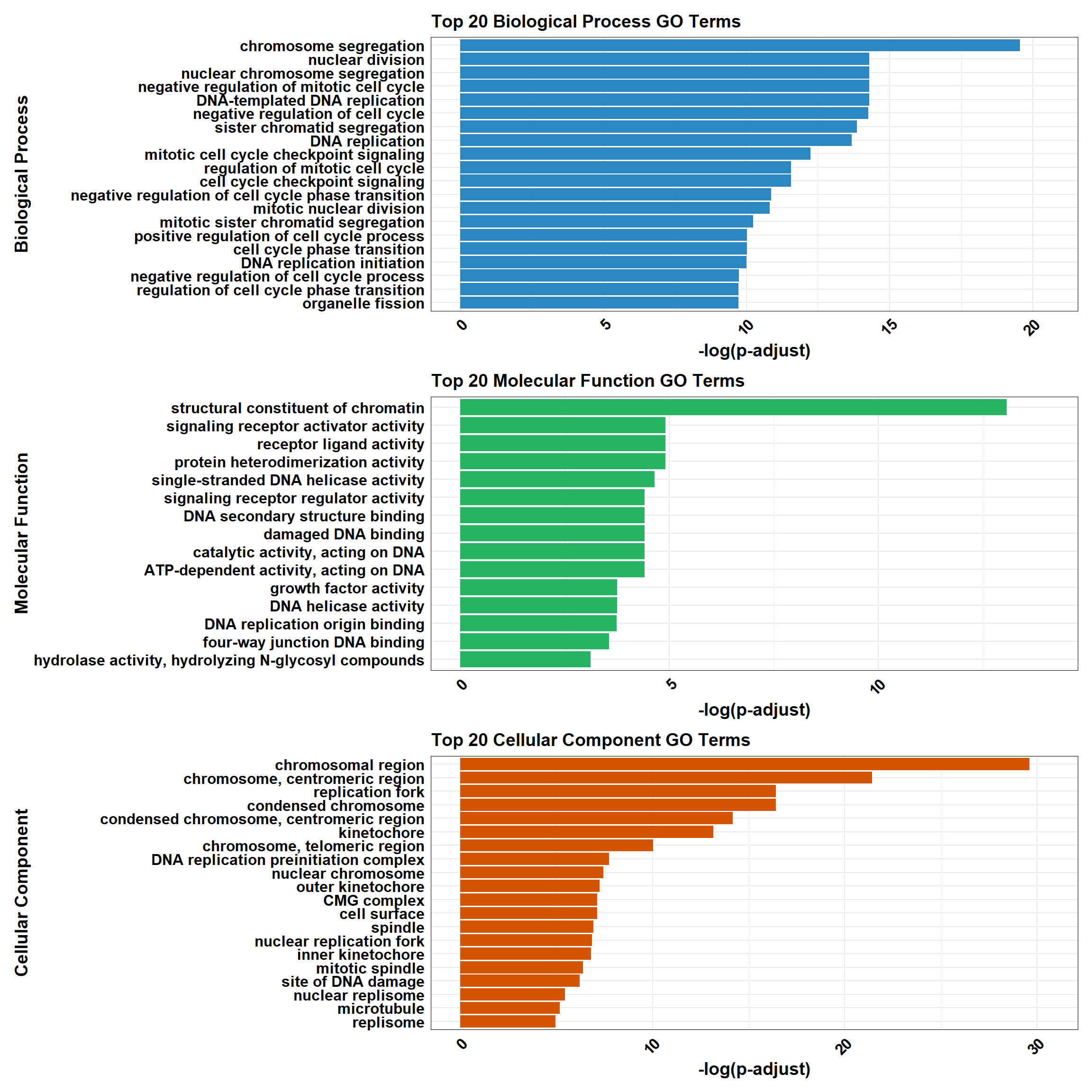
📌 DOX vs VEH (0.1 and 24hr) GO Enrichment g:Profiler
# Load the gprofiler2 package
library(gprofiler2)
library(ggplot2)
library(dplyr)
library(patchwork)

# Perform GO enrichment analysis with gprofiler2
gost_results <- gost(
  query = DEG8,
  organism = "hsapiens",   # Human organism
  user_threshold = 0.05,   # Adjusted p-value cutoff
  correction_method = "fdr", # Multiple testing correction
  domain_scope = "custom", # Use custom background
  custom_bg = background,    # Background set of genes
  sources = c("GO:BP", "GO:MF", "GO:CC") # Analyze GO categories
)

# Check if enrichment results exist
if (is.null(gost_results$result) || nrow(gost_results$result) == 0) {
  # If no enriched terms, create a placeholder dataframe
  combined_results <- tibble(
    term_name = "No enriched terms",
    p.adjust = NA,
    source = "N/A",
    Category = "N/A"
  )
} else {
  # Convert results to a data frame
  gost_results_df <- gost_results$result

  # Add a column for adjusted p-value
  gost_results_df <- gost_results_df %>%
    rename(p.adjust = p_value)

  # Separate results for BP, MF, and CC
  BP_results <- gost_results_df %>%
    filter(source == "GO:BP") %>%
    mutate(Category = "Biological Process")

  MF_results <- gost_results_df %>%
    filter(source == "GO:MF") %>%
    mutate(Category = "Molecular Function")

  CC_results <- gost_results_df %>%
    filter(source == "GO:CC") %>%
    mutate(Category = "Cellular Component")

  # Select the top 20 terms by adjusted p-value for each category
  top_BP <- BP_results %>%
    arrange(p.adjust) %>%
    slice_head(n = 20)

  top_MF <- MF_results %>%
    arrange(p.adjust) %>%
    slice_head(n = 20)

  top_CC <- CC_results %>%
    arrange(p.adjust) %>%
    slice_head(n = 20)

  # Combine all categories
  combined_results <- bind_rows(top_BP, top_MF, top_CC)
}

# Ensure all columns are atomic types for CSV export
combined_results_clean <- combined_results %>%
  mutate(across(everything(), ~ if (is.list(.)) sapply(., toString) else .))

# Function for plotting top terms
plot_gprofiler_results <- function(data, title, color) {
  ggplot(data, aes(x = -log10(p.adjust), y = reorder(term_name, -log10(p.adjust)))) +
    geom_bar(stat = "identity", fill = color) +
    labs(
      x = "-log10(Adjusted p-value)",
      y = title,
      title = paste("Top 20", title, "GO Terms")
    ) +
    theme_minimal() +
    theme(
      axis.text.x = element_text(size = 12, face = "bold", colour = "black", angle = 45, hjust = 1),
      axis.text.y = element_text(size = 12, face = "bold", colour = "black"),
      axis.title.x = element_text(size = 14, face = "bold", colour = "black"),
      axis.title.y = element_text(size = 14, face = "bold", colour = "black"),
      plot.title = element_text(size = 14, face = "bold", colour = "black"),
      panel.border = element_rect(colour = "black", fill = NA, size = 0.3)
    )
}

# Check if there are enrichment terms to plot
if (nrow(combined_results) == 1 && combined_results$term_name == "No enriched terms") {
  message("No enriched GO terms found for the input gene set.")
} else {
  # Plot the top 20 terms for each category
  plot_BP <- plot_gprofiler_results(top_BP, "Biological Process", "#2E86C1")
  plot_MF <- plot_gprofiler_results(top_MF, "Molecular Function", "#28B463")
  plot_CC <- plot_gprofiler_results(top_CC, "Cellular Component", "#D35400")

  # Combine the plots using patchwork
  combined_plot <- plot_BP / plot_MF / plot_CC

  # Display the combined plot
  combined_plot
}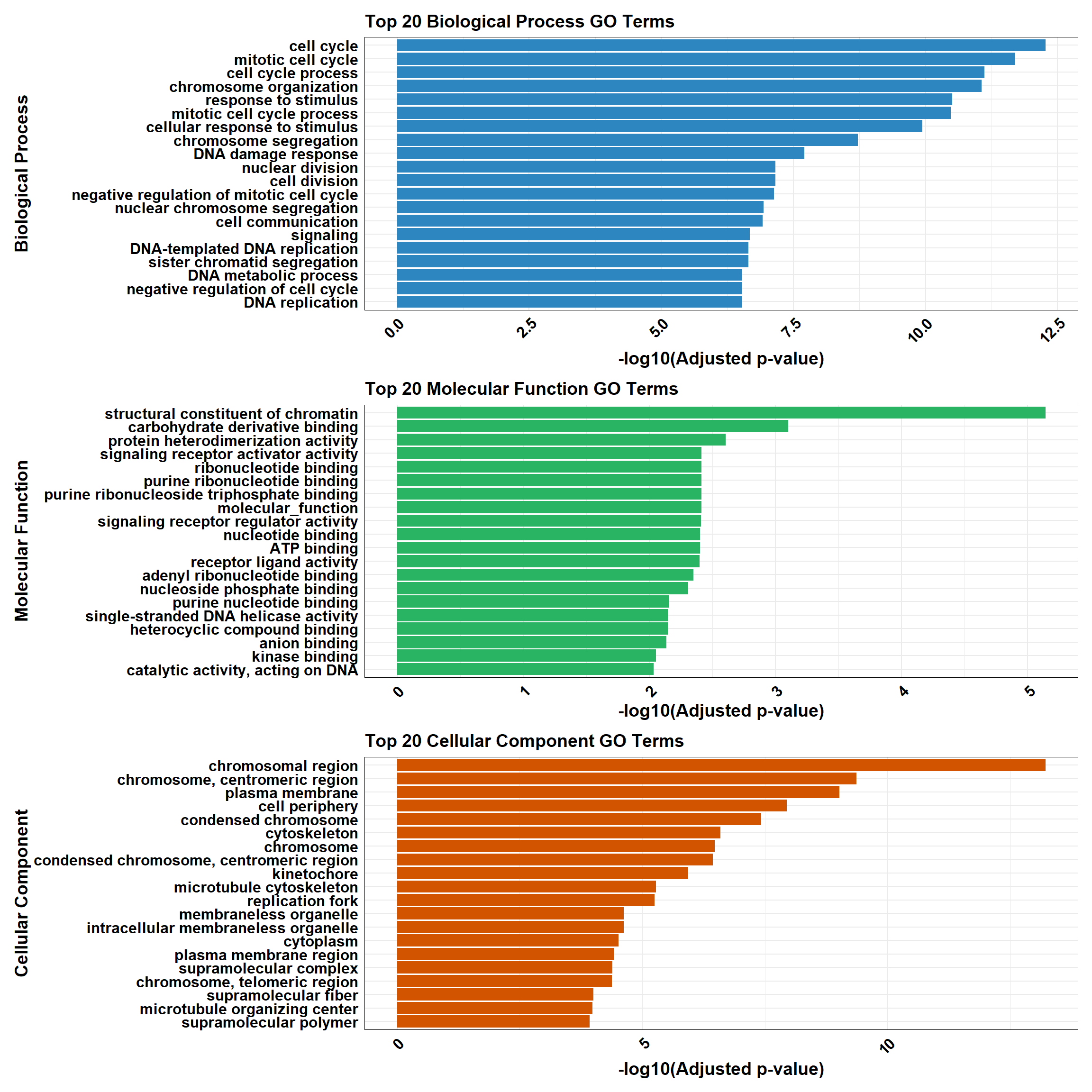
📌 DOX vs VEH (0.1 and 24hr) Pathway Enrichment
# Load required libraries
library(clusterProfiler)
library(org.Hs.eg.db) # Required for enrichPathway
library(gprofiler2)
library(ggplot2)
library(dplyr)
library(patchwork)
library(ReactomePA)

# Function for ClusterProfiler Reactome & KEGG Analysis
process_clusterProfiler <- function(gene_set, background, category, color, y_title) {
  # Perform enrichment based on the selected category
  if (category == "Reactome") {
    enrichment <- enrichPathway(
      gene = gene_set,
      organism = "human",
      pvalueCutoff = 0.05,
      pAdjustMethod = "BH",
      universe = background
    )
  } else if (category == "KEGG") {
    enrichment <- enrichKEGG(
      gene = gene_set,
      organism = "hsa",
      pvalueCutoff = 0.05,
      pAdjustMethod = "BH",
      universe = background
    )
  }

  # Check if enrichment results exist
  if (is.null(enrichment) || nrow(as.data.frame(enrichment)) == 0) {
    message(paste("No significant enrichment found for", category, "in ClusterProfiler"))
    return(NULL)
  }

  # Convert results to tibble and process top 20 terms
  enrichment_tibble <- as_tibble(as.data.frame(enrichment)) %>%
    mutate(Category = category,
           neglog = -log10(p.adjust)) %>%  # Compute -log10(p.adjust)
    arrange(desc(neglog)) %>%
    slice_head(n = min(20, nrow(.)))  # Ensure safe slicing

  # Generate plot
  plot <- ggplot(enrichment_tibble, aes(x = neglog, y = reorder(Description, neglog))) +
    geom_bar(stat = "identity", fill = color) +
    labs(x = "-log10(Adjusted p-value)",
         y = y_title,
         title = paste("Enriched", category, "Pathways")) +
    theme_minimal() +
    theme(
      axis.text.x = element_text(size = 12, face = "bold", colour = "black", angle = 45, hjust = 1),
      axis.text.y = element_text(size = 12, face = "bold", colour = "black"),
      axis.title.x = element_text(size = 14, face = "bold", colour = "black"),
      axis.title.y = element_text(size = 14, face = "bold", colour = "black"),
      plot.title = element_text(size = 14, face = "bold", colour = "black")
    )

  return(plot)
}

# Function for gProfiler Reactome & KEGG Analysis
process_gprofiler <- function(gene_set, background, category, color, y_title) {
  # Perform enrichment using gprofiler2
  enrichment <- gost(
    query = gene_set,
    organism = "hsapiens",
    user_threshold = 0.05,
    correction_method = "fdr",
    domain_scope = "custom",
    custom_bg = background,
    sources = category # Either "REAC" or "KEGG"
  )

  # Check if enrichment results exist
  if (is.null(enrichment$result) || nrow(enrichment$result) == 0) {
    message(paste("No significant enrichment found for", category, "in gProfiler"))
    return(NULL)
  }

  # Convert results to tibble and process top 20 terms
  enrichment_tibble <- enrichment$result %>%
    as_tibble() %>%
    mutate(Category = category,
           neglog = -log10(p_value)) %>%  # Compute -log10(p-value)
    arrange(desc(neglog)) %>%
    slice_head(n = min(20, nrow(.)))  # Ensure safe slicing

  # Generate plot
  plot <- ggplot(enrichment_tibble, aes(x = neglog, y = reorder(term_name, neglog))) +
    geom_bar(stat = "identity", fill = color) +
    labs(x = "-log10(p-value)",
         y = y_title,
         title = paste("Enriched", category, "Pathways")) +
    theme_minimal() +
    theme(
      axis.text.x = element_text(size = 12, face = "bold", colour = "black", angle = 45, hjust = 1),
      axis.text.y = element_text(size = 12, face = "bold", colour = "black"),
      axis.title.x = element_text(size = 14, face = "bold", colour = "black"),
      axis.title.y = element_text(size = 14, face = "bold", colour = "black"),
      plot.title = element_text(size = 14, face = "bold", colour = "black")
    )

  return(plot)
}

# Perform analysis for Reactome and KEGG using ClusterProfiler
cluster_reactome <- process_clusterProfiler(
  gene_set = DEG8,
  background = background,
  category = "Reactome",
  color = "#2E86C1",
  y_title = "Reactome Pathways"
)

cluster_kegg <- process_clusterProfiler(
  gene_set = DEG8,
  background = background,
  category = "KEGG",
  color = "#28B463",
  y_title = "KEGG Pathways"
)

# Combine Reactome and KEGG for ClusterProfiler
if (!is.null(cluster_reactome) && !is.null(cluster_kegg)) {
  cluster_combined <- cluster_reactome / cluster_kegg
} else if (!is.null(cluster_reactome)) {
  cluster_combined <- cluster_reactome
} else if (!is.null(cluster_kegg)) {
  cluster_combined <- cluster_kegg
} else {
  cluster_combined <- NULL
}

# Perform analysis for Reactome and KEGG using GProfiler
gprofiler_reactome <- process_gprofiler(
  gene_set = DEG8,
  background = background,
  category = "REAC",  # Corrected category for Reactome in gProfiler
  color = "#D35400",
  y_title = "Reactome Pathways"
)

gprofiler_kegg <- process_gprofiler(
  gene_set = DEG8,
  background = background,
  category = "KEGG",
  color = "#F39C12",
  y_title = "KEGG Pathways"
)

# Combine Reactome and KEGG for GProfiler
if (!is.null(gprofiler_reactome) && !is.null(gprofiler_kegg)) {
  gprofiler_combined <- gprofiler_reactome / gprofiler_kegg
} else if (!is.null(gprofiler_reactome)) {
  gprofiler_combined <- gprofiler_reactome
} else if (!is.null(gprofiler_kegg)) {
  gprofiler_combined <- gprofiler_kegg
} else {
  gprofiler_combined <- NULL
}

# Display plots (if they are not NULL)
if (!is.null(cluster_combined)) print(cluster_combined)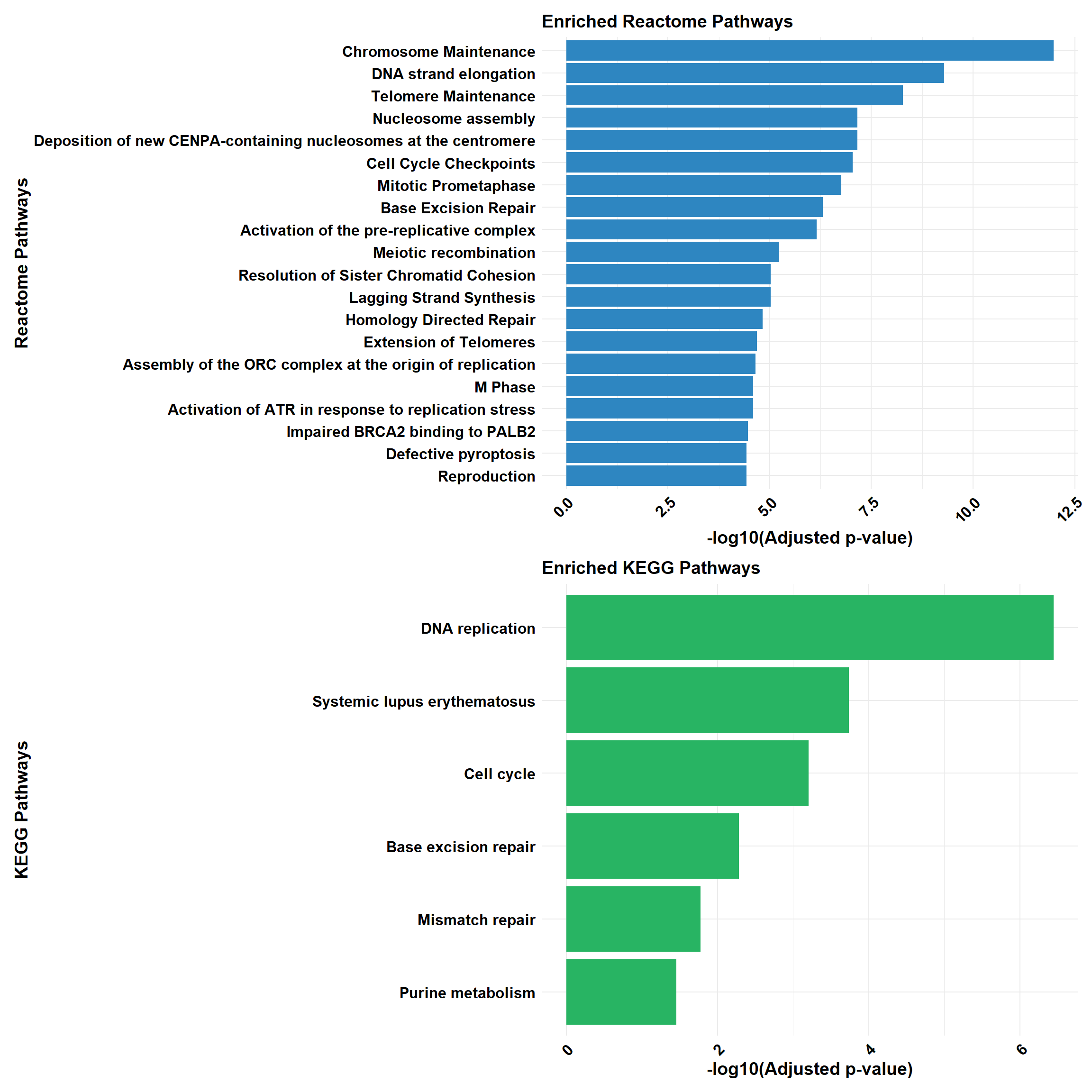
if (!is.null(gprofiler_combined)) print(gprofiler_combined)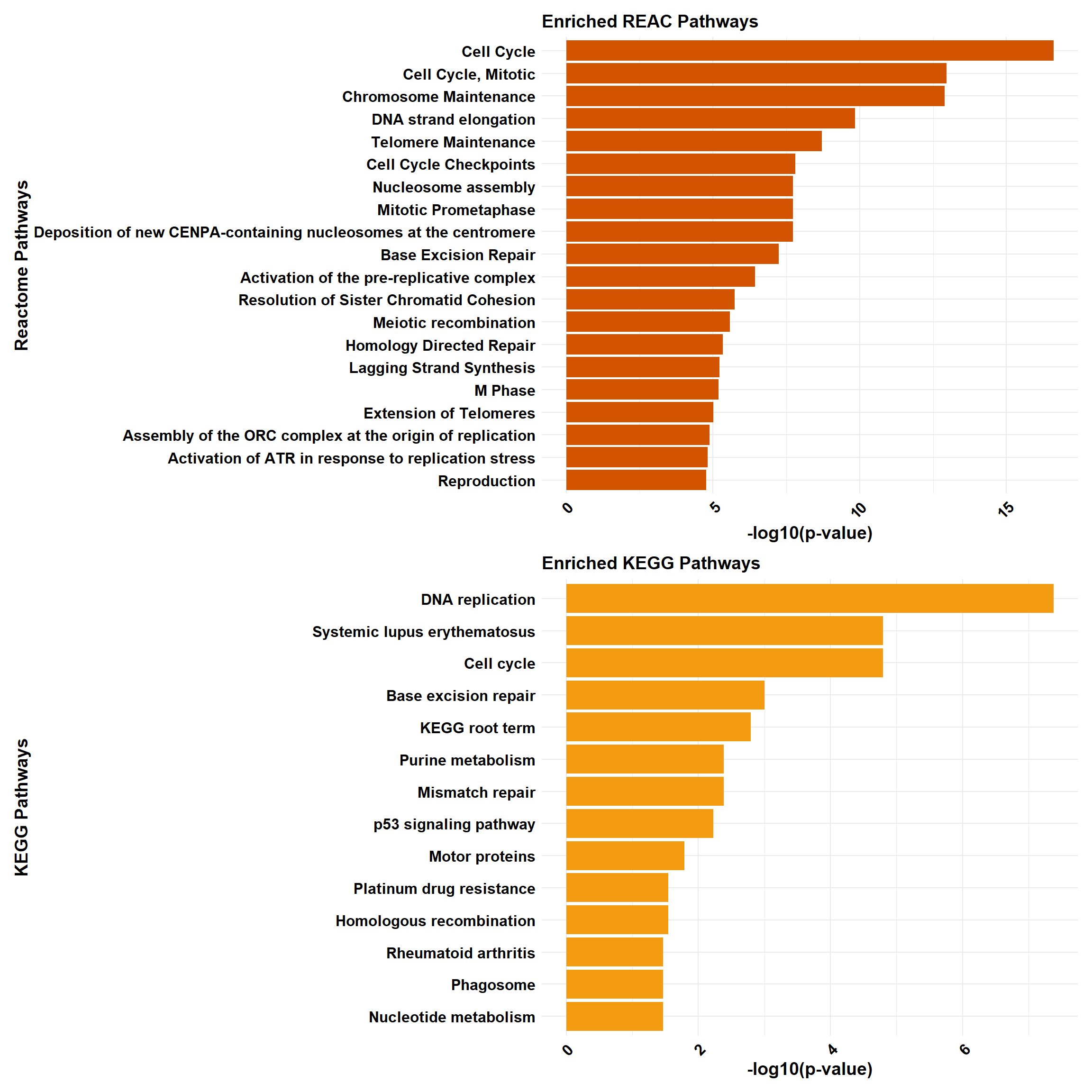
📌 DOX vs VEH (0.1 and 48hr)
📌 DOX vs VEH (0.1 and 48hr) GO Enrichment Clusterprofiler
# Perform GO enrichment analysis for BP, MF, and CC
go_enrichment_BP <- enrichGO(gene = DEG9,
                             OrgDb = org.Hs.eg.db,
                             keyType = "ENTREZID",
                             universe = background,
                             ont = "BP",
                             pvalueCutoff = 0.05)

go_enrichment_MF <- enrichGO(gene = DEG9,
                             OrgDb = org.Hs.eg.db,
                             keyType = "ENTREZID",
                             universe = background,
                             ont = "MF",
                             pvalueCutoff = 0.05)

go_enrichment_CC <- enrichGO(gene = DEG9,
                             OrgDb = org.Hs.eg.db,
                             keyType = "ENTREZID",
                             universe = background,
                             ont = "CC",
                             pvalueCutoff = 0.05)

# Convert each enrichment result to a tibble, add a category column, and select top 20 terms
process_enrichment_tibble <- function(enrichment, category) {
  if (is.null(enrichment) || nrow(as.data.frame(enrichment)) == 0) {
    return(tibble(Description = "No enriched terms", neglog = 0, Category = category))
  } else {
    enrichment %>%
      as_tibble() %>%
      mutate(Category = category,
             neglog = -log(p.adjust)) %>% # Add -log(p.adjust) column
      arrange(desc(neglog)) %>%          # Sort by -log(p.adjust)
      slice(1:20)                        # Select top 20 terms
  }
}

BP_Tibble <- process_enrichment_tibble(go_enrichment_BP, "Biological Process")
MF_Tibble <- process_enrichment_tibble(go_enrichment_MF, "Molecular Function")
CC_Tibble <- process_enrichment_tibble(go_enrichment_CC, "Cellular Component")

# Combine all tibbles
combined_GO_Tibble <- bind_rows(BP_Tibble, MF_Tibble, CC_Tibble)
# Function to generate enrichment plots
process_enrichment_plot <- function(tibble, title, color) {
  ggplot(data = tibble, aes(x = neglog, y = reorder(Description, neglog))) +
    geom_bar(stat = "identity", fill = color) +
    labs(x = "-log(p-adjust)",
         y = title,
         title = paste("Top 20", title, "GO Terms")) +
    theme_minimal() +
    theme(
      axis.text.x = element_text(size = 12, face = "bold", colour = "black", angle = 45, hjust = 1),
      axis.text.y = element_text(size = 12, face = "bold", colour = "black"),
      axis.title.x = element_text(size = 14, face = "bold", colour = "black"),
      axis.title.y = element_text(size = 14, face = "bold", colour = "black"),
      plot.title = element_text(size = 14, face = "bold", colour = "black"),
      panel.border = element_rect(colour = "black", fill = NA, size = 0.3)
    ) +
    xlim(c(0, max(tibble$neglog) + 1))
}

# Generate separate plots
plot_BP <- process_enrichment_plot(BP_Tibble, "Biological Process", "#2E86C1")
plot_MF <- process_enrichment_plot(MF_Tibble, "Molecular Function", "#28B463")
plot_CC <- process_enrichment_plot(CC_Tibble, "Cellular Component", "#D35400")

# Combine the plots using patchwork
combined_plot <- plot_BP / plot_MF / plot_CC

# Display the combined plot
combined_plot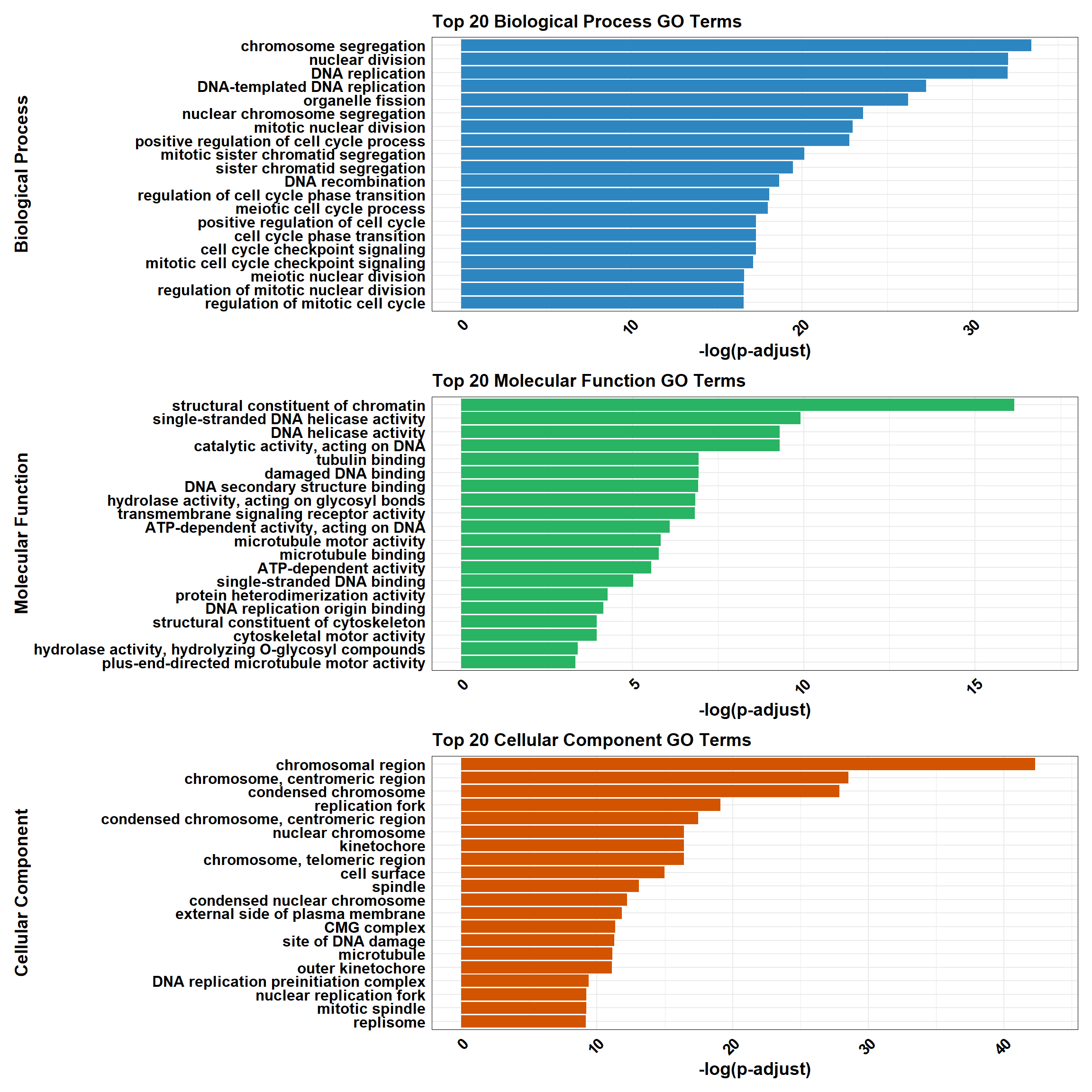
📌 DOX vs VEH (0.1 and 48hr) GO Enrichment g:Profiler
# Load the gprofiler2 package
library(gprofiler2)
library(ggplot2)
library(dplyr)
library(patchwork)

# Perform GO enrichment analysis with gprofiler2
gost_results <- gost(
  query = DEG9,
  organism = "hsapiens",   # Human organism
  user_threshold = 0.05,   # Adjusted p-value cutoff
  correction_method = "fdr", # Multiple testing correction
  domain_scope = "custom", # Use custom background
  custom_bg = background,    # Background set of genes
  sources = c("GO:BP", "GO:MF", "GO:CC") # Analyze GO categories
)

# Check if enrichment results exist
if (is.null(gost_results$result) || nrow(gost_results$result) == 0) {
  # If no enriched terms, create a placeholder dataframe
  combined_results <- tibble(
    term_name = "No enriched terms",
    p.adjust = NA,
    source = "N/A",
    Category = "N/A"
  )
} else {
  # Convert results to a data frame
  gost_results_df <- gost_results$result

  # Add a column for adjusted p-value
  gost_results_df <- gost_results_df %>%
    rename(p.adjust = p_value)

  # Separate results for BP, MF, and CC
  BP_results <- gost_results_df %>%
    filter(source == "GO:BP") %>%
    mutate(Category = "Biological Process")

  MF_results <- gost_results_df %>%
    filter(source == "GO:MF") %>%
    mutate(Category = "Molecular Function")

  CC_results <- gost_results_df %>%
    filter(source == "GO:CC") %>%
    mutate(Category = "Cellular Component")

  # Select the top 20 terms by adjusted p-value for each category
  top_BP <- BP_results %>%
    arrange(p.adjust) %>%
    slice_head(n = 20)

  top_MF <- MF_results %>%
    arrange(p.adjust) %>%
    slice_head(n = 20)

  top_CC <- CC_results %>%
    arrange(p.adjust) %>%
    slice_head(n = 20)

  # Combine all categories
  combined_results <- bind_rows(top_BP, top_MF, top_CC)
}

# Ensure all columns are atomic types for CSV export
combined_results_clean <- combined_results %>%
  mutate(across(everything(), ~ if (is.list(.)) sapply(., toString) else .))

# Function for plotting top terms
plot_gprofiler_results <- function(data, title, color) {
  ggplot(data, aes(x = -log10(p.adjust), y = reorder(term_name, -log10(p.adjust)))) +
    geom_bar(stat = "identity", fill = color) +
    labs(
      x = "-log10(Adjusted p-value)",
      y = title,
      title = paste("Top 20", title, "GO Terms")
    ) +
    theme_minimal() +
    theme(
      axis.text.x = element_text(size = 12, face = "bold", colour = "black", angle = 45, hjust = 1),
      axis.text.y = element_text(size = 12, face = "bold", colour = "black"),
      axis.title.x = element_text(size = 14, face = "bold", colour = "black"),
      axis.title.y = element_text(size = 14, face = "bold", colour = "black"),
      plot.title = element_text(size = 14, face = "bold", colour = "black"),
      panel.border = element_rect(colour = "black", fill = NA, size = 0.3)
    )
}

# Check if there are enrichment terms to plot
if (nrow(combined_results) == 1 && combined_results$term_name == "No enriched terms") {
  message("No enriched GO terms found for the input gene set.")
} else {
  # Plot the top 20 terms for each category
  plot_BP <- plot_gprofiler_results(top_BP, "Biological Process", "#2E86C1")
  plot_MF <- plot_gprofiler_results(top_MF, "Molecular Function", "#28B463")
  plot_CC <- plot_gprofiler_results(top_CC, "Cellular Component", "#D35400")

  # Combine the plots using patchwork
  combined_plot <- plot_BP / plot_MF / plot_CC

  # Display the combined plot
  combined_plot
}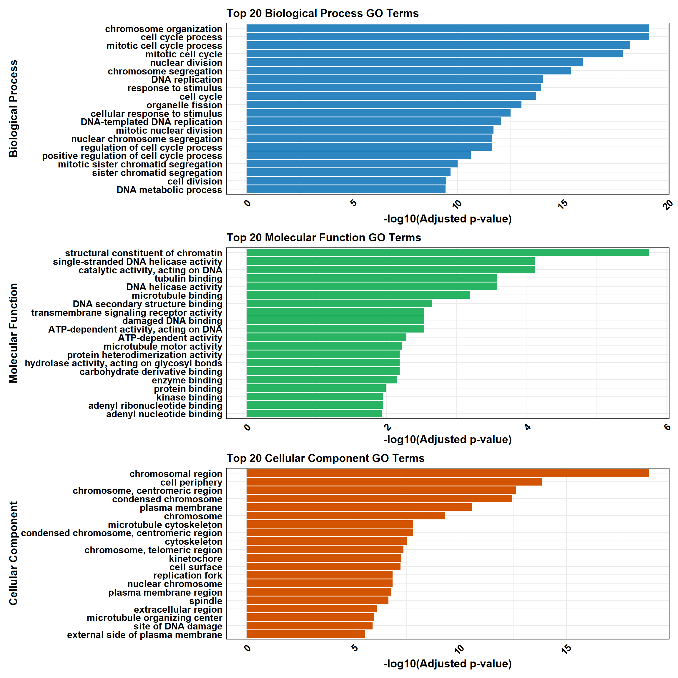
📌 DOX vs VEH (0.1 and 48hr) Pathway Enrichment
# Load required libraries
library(clusterProfiler)
library(org.Hs.eg.db) # Required for enrichPathway
library(gprofiler2)
library(ggplot2)
library(dplyr)
library(patchwork)
library(ReactomePA)

# Function for ClusterProfiler Reactome & KEGG Analysis
process_clusterProfiler <- function(gene_set, background, category, color, y_title) {
  # Perform enrichment based on the selected category
  if (category == "Reactome") {
    enrichment <- enrichPathway(
      gene = gene_set,
      organism = "human",
      pvalueCutoff = 0.05,
      pAdjustMethod = "BH",
      universe = background
    )
  } else if (category == "KEGG") {
    enrichment <- enrichKEGG(
      gene = gene_set,
      organism = "hsa",
      pvalueCutoff = 0.05,
      pAdjustMethod = "BH",
      universe = background
    )
  }

  # Check if enrichment results exist
  if (is.null(enrichment) || nrow(as.data.frame(enrichment)) == 0) {
    message(paste("No significant enrichment found for", category, "in ClusterProfiler"))
    return(NULL)
  }

  # Convert results to tibble and process top 20 terms
  enrichment_tibble <- as_tibble(as.data.frame(enrichment)) %>%
    mutate(Category = category,
           neglog = -log10(p.adjust)) %>%  # Compute -log10(p.adjust)
    arrange(desc(neglog)) %>%
    slice_head(n = min(20, nrow(.)))  # Ensure safe slicing

  # Generate plot
  plot <- ggplot(enrichment_tibble, aes(x = neglog, y = reorder(Description, neglog))) +
    geom_bar(stat = "identity", fill = color) +
    labs(x = "-log10(Adjusted p-value)",
         y = y_title,
         title = paste("Enriched", category, "Pathways")) +
    theme_minimal() +
    theme(
      axis.text.x = element_text(size = 12, face = "bold", colour = "black", angle = 45, hjust = 1),
      axis.text.y = element_text(size = 12, face = "bold", colour = "black"),
      axis.title.x = element_text(size = 14, face = "bold", colour = "black"),
      axis.title.y = element_text(size = 14, face = "bold", colour = "black"),
      plot.title = element_text(size = 14, face = "bold", colour = "black")
    )

  return(plot)
}

# Function for gProfiler Reactome & KEGG Analysis
process_gprofiler <- function(gene_set, background, category, color, y_title) {
  # Perform enrichment using gprofiler2
  enrichment <- gost(
    query = gene_set,
    organism = "hsapiens",
    user_threshold = 0.05,
    correction_method = "fdr",
    domain_scope = "custom",
    custom_bg = background,
    sources = category # Either "REAC" or "KEGG"
  )

  # Check if enrichment results exist
  if (is.null(enrichment$result) || nrow(enrichment$result) == 0) {
    message(paste("No significant enrichment found for", category, "in gProfiler"))
    return(NULL)
  }

  # Convert results to tibble and process top 20 terms
  enrichment_tibble <- enrichment$result %>%
    as_tibble() %>%
    mutate(Category = category,
           neglog = -log10(p_value)) %>%  # Compute -log10(p-value)
    arrange(desc(neglog)) %>%
    slice_head(n = min(20, nrow(.)))  # Ensure safe slicing

  # Generate plot
  plot <- ggplot(enrichment_tibble, aes(x = neglog, y = reorder(term_name, neglog))) +
    geom_bar(stat = "identity", fill = color) +
    labs(x = "-log10(p-value)",
         y = y_title,
         title = paste("Enriched", category, "Pathways")) +
    theme_minimal() +
    theme(
      axis.text.x = element_text(size = 12, face = "bold", colour = "black", angle = 45, hjust = 1),
      axis.text.y = element_text(size = 12, face = "bold", colour = "black"),
      axis.title.x = element_text(size = 14, face = "bold", colour = "black"),
      axis.title.y = element_text(size = 14, face = "bold", colour = "black"),
      plot.title = element_text(size = 14, face = "bold", colour = "black")
    )

  return(plot)
}

# Perform analysis for Reactome and KEGG using ClusterProfiler
cluster_reactome <- process_clusterProfiler(
  gene_set = DEG9,
  background = background,
  category = "Reactome",
  color = "#2E86C1",
  y_title = "Reactome Pathways"
)

cluster_kegg <- process_clusterProfiler(
  gene_set = DEG9,
  background = background,
  category = "KEGG",
  color = "#28B463",
  y_title = "KEGG Pathways"
)

# Combine Reactome and KEGG for ClusterProfiler
if (!is.null(cluster_reactome) && !is.null(cluster_kegg)) {
  cluster_combined <- cluster_reactome / cluster_kegg
} else if (!is.null(cluster_reactome)) {
  cluster_combined <- cluster_reactome
} else if (!is.null(cluster_kegg)) {
  cluster_combined <- cluster_kegg
} else {
  cluster_combined <- NULL
}

# Perform analysis for Reactome and KEGG using GProfiler
gprofiler_reactome <- process_gprofiler(
  gene_set = DEG9,
  background = background,
  category = "REAC",  # Corrected category for Reactome in gProfiler
  color = "#D35400",
  y_title = "Reactome Pathways"
)

gprofiler_kegg <- process_gprofiler(
  gene_set = DEG9,
  background = background,
  category = "KEGG",
  color = "#F39C12",
  y_title = "KEGG Pathways"
)

# Combine Reactome and KEGG for GProfiler
if (!is.null(gprofiler_reactome) && !is.null(gprofiler_kegg)) {
  gprofiler_combined <- gprofiler_reactome / gprofiler_kegg
} else if (!is.null(gprofiler_reactome)) {
  gprofiler_combined <- gprofiler_reactome
} else if (!is.null(gprofiler_kegg)) {
  gprofiler_combined <- gprofiler_kegg
} else {
  gprofiler_combined <- NULL
}

# Display plots (if they are not NULL)
if (!is.null(cluster_combined)) print(cluster_combined)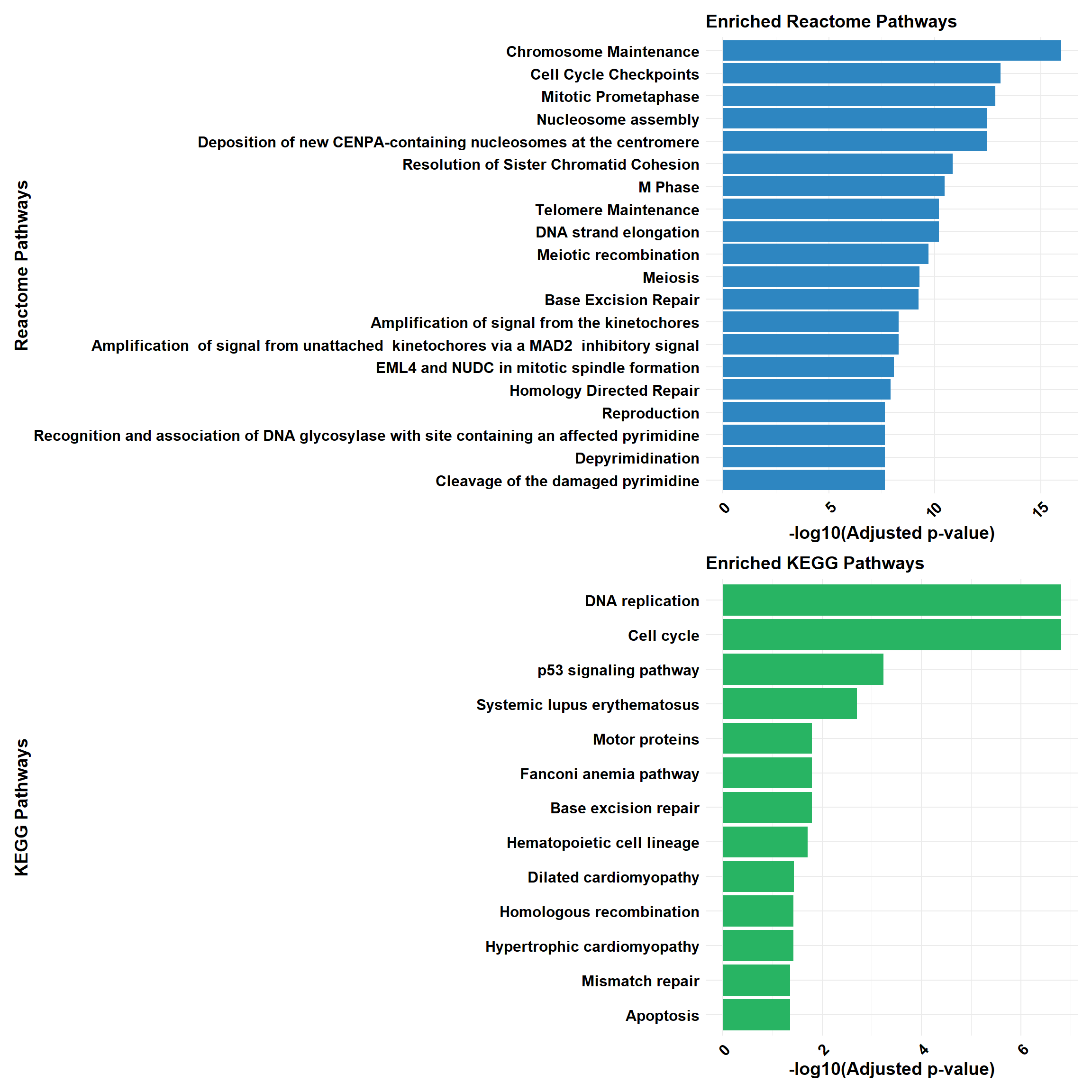
if (!is.null(gprofiler_combined)) print(gprofiler_combined)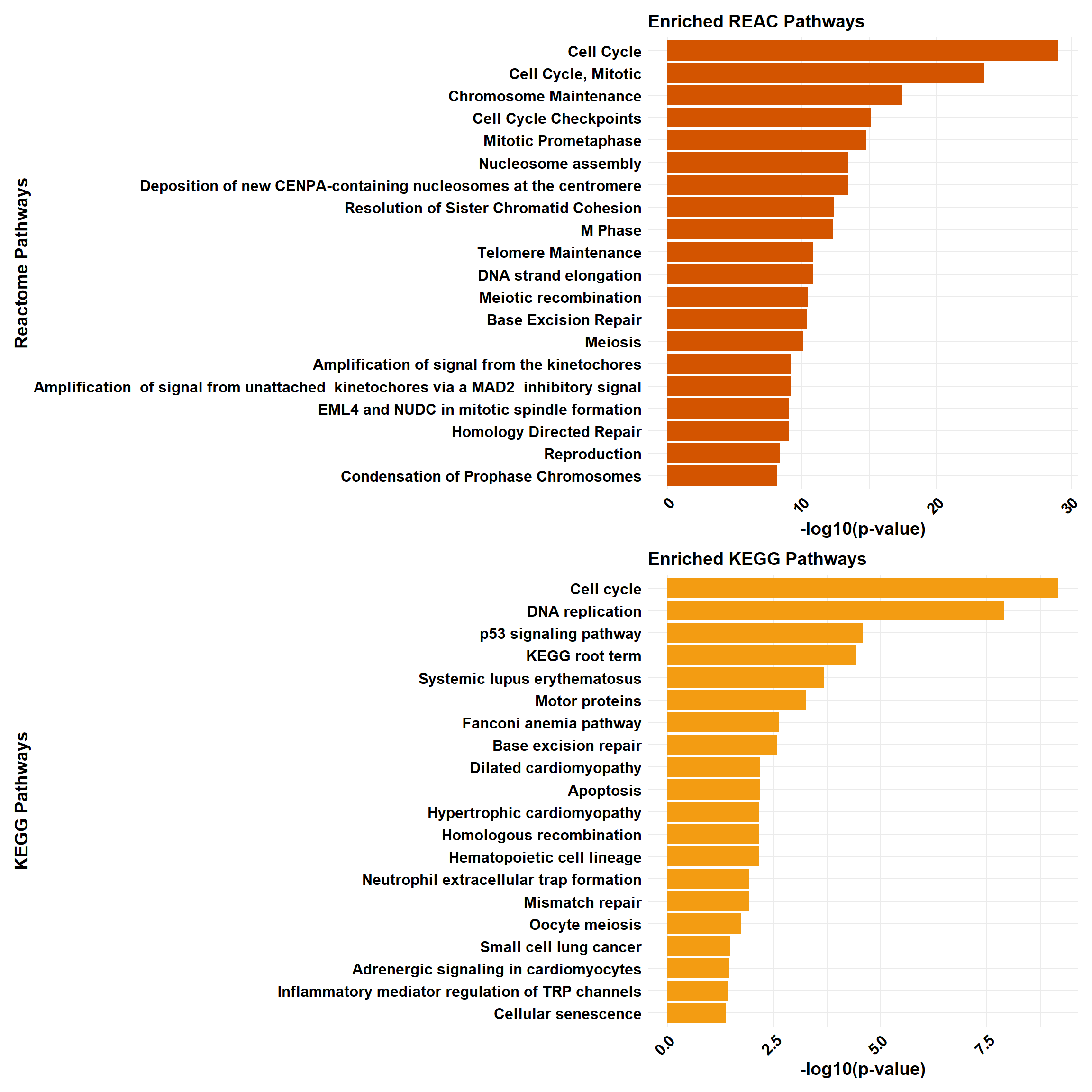
📌 DOX vs VEH (0.5 and 3hr)
📌 DOX vs VEH (0.5 and 3hr) GO Enrichment Clusterprofiler
# Perform GO enrichment analysis for BP, MF, and CC
go_enrichment_BP <- enrichGO(gene = DEG10,
                             OrgDb = org.Hs.eg.db,
                             keyType = "ENTREZID",
                             universe = background,
                             ont = "BP",
                             pvalueCutoff = 0.05)

go_enrichment_MF <- enrichGO(gene = DEG10,
                             OrgDb = org.Hs.eg.db,
                             keyType = "ENTREZID",
                             universe = background,
                             ont = "MF",
                             pvalueCutoff = 0.05)

go_enrichment_CC <- enrichGO(gene = DEG10,
                             OrgDb = org.Hs.eg.db,
                             keyType = "ENTREZID",
                             universe = background,
                             ont = "CC",
                             pvalueCutoff = 0.05)

# Convert each enrichment result to a tibble, add a category column, and select top 20 terms
process_enrichment_tibble <- function(enrichment, category) {
  if (is.null(enrichment) || nrow(as.data.frame(enrichment)) == 0) {
    return(tibble(Description = "No enriched terms", neglog = 0, Category = category))
  } else {
    enrichment %>%
      as_tibble() %>%
      mutate(Category = category,
             neglog = -log(p.adjust)) %>% # Add -log(p.adjust) column
      arrange(desc(neglog)) %>%          # Sort by -log(p.adjust)
      slice(1:20)                        # Select top 20 terms
  }
}

BP_Tibble <- process_enrichment_tibble(go_enrichment_BP, "Biological Process")
MF_Tibble <- process_enrichment_tibble(go_enrichment_MF, "Molecular Function")
CC_Tibble <- process_enrichment_tibble(go_enrichment_CC, "Cellular Component")

# Combine all tibbles
combined_GO_Tibble <- bind_rows(BP_Tibble, MF_Tibble, CC_Tibble)
# Function to generate enrichment plots
process_enrichment_plot <- function(tibble, title, color) {
  ggplot(data = tibble, aes(x = neglog, y = reorder(Description, neglog))) +
    geom_bar(stat = "identity", fill = color) +
    labs(x = "-log(p-adjust)",
         y = title,
         title = paste("Top 20", title, "GO Terms")) +
    theme_minimal() +
    theme(
      axis.text.x = element_text(size = 12, face = "bold", colour = "black", angle = 45, hjust = 1),
      axis.text.y = element_text(size = 12, face = "bold", colour = "black"),
      axis.title.x = element_text(size = 14, face = "bold", colour = "black"),
      axis.title.y = element_text(size = 14, face = "bold", colour = "black"),
      plot.title = element_text(size = 14, face = "bold", colour = "black"),
      panel.border = element_rect(colour = "black", fill = NA, size = 0.3)
    ) +
    xlim(c(0, max(tibble$neglog) + 1))
}

# Generate separate plots
plot_BP <- process_enrichment_plot(BP_Tibble, "Biological Process", "#2E86C1")
plot_MF <- process_enrichment_plot(MF_Tibble, "Molecular Function", "#28B463")
plot_CC <- process_enrichment_plot(CC_Tibble, "Cellular Component", "#D35400")

# Combine the plots using patchwork
combined_plot <- plot_BP / plot_MF / plot_CC

# Display the combined plot
combined_plot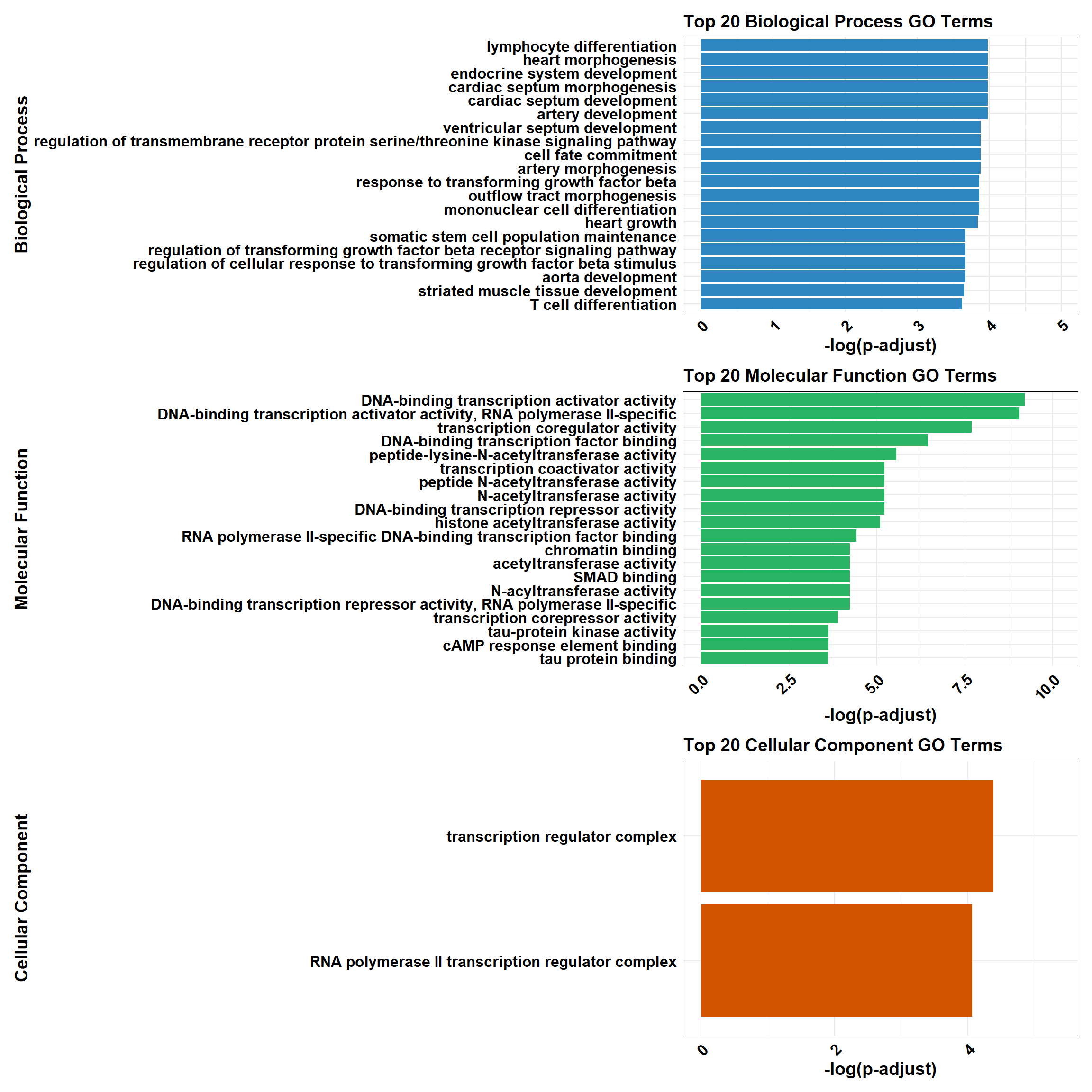
📌 DOX vs VEH (0.5 and 3hr) GO Enrichment g:Profiler
# Load the gprofiler2 package
library(gprofiler2)
library(ggplot2)
library(dplyr)
library(patchwork)

# Perform GO enrichment analysis with gprofiler2
gost_results <- gost(
  query = DEG10,
  organism = "hsapiens",   # Human organism
  user_threshold = 0.05,   # Adjusted p-value cutoff
  correction_method = "fdr", # Multiple testing correction
  domain_scope = "custom", # Use custom background
  custom_bg = background,    # Background set of genes
  sources = c("GO:BP", "GO:MF", "GO:CC") # Analyze GO categories
)

# Check if enrichment results exist
if (is.null(gost_results$result) || nrow(gost_results$result) == 0) {
  # If no enriched terms, create a placeholder dataframe
  combined_results <- tibble(
    term_name = "No enriched terms",
    p.adjust = NA,
    source = "N/A",
    Category = "N/A"
  )
} else {
  # Convert results to a data frame
  gost_results_df <- gost_results$result

  # Add a column for adjusted p-value
  gost_results_df <- gost_results_df %>%
    rename(p.adjust = p_value)

  # Separate results for BP, MF, and CC
  BP_results <- gost_results_df %>%
    filter(source == "GO:BP") %>%
    mutate(Category = "Biological Process")

  MF_results <- gost_results_df %>%
    filter(source == "GO:MF") %>%
    mutate(Category = "Molecular Function")

  CC_results <- gost_results_df %>%
    filter(source == "GO:CC") %>%
    mutate(Category = "Cellular Component")

  # Select the top 20 terms by adjusted p-value for each category
  top_BP <- BP_results %>%
    arrange(p.adjust) %>%
    slice_head(n = 20)

  top_MF <- MF_results %>%
    arrange(p.adjust) %>%
    slice_head(n = 20)

  top_CC <- CC_results %>%
    arrange(p.adjust) %>%
    slice_head(n = 20)

  # Combine all categories
  combined_results <- bind_rows(top_BP, top_MF, top_CC)
}

# Ensure all columns are atomic types for CSV export
combined_results_clean <- combined_results %>%
  mutate(across(everything(), ~ if (is.list(.)) sapply(., toString) else .))

# Function for plotting top terms
plot_gprofiler_results <- function(data, title, color) {
  ggplot(data, aes(x = -log10(p.adjust), y = reorder(term_name, -log10(p.adjust)))) +
    geom_bar(stat = "identity", fill = color) +
    labs(
      x = "-log10(Adjusted p-value)",
      y = title,
      title = paste("Top 20", title, "GO Terms")
    ) +
    theme_minimal() +
    theme(
      axis.text.x = element_text(size = 12, face = "bold", colour = "black", angle = 45, hjust = 1),
      axis.text.y = element_text(size = 12, face = "bold", colour = "black"),
      axis.title.x = element_text(size = 14, face = "bold", colour = "black"),
      axis.title.y = element_text(size = 14, face = "bold", colour = "black"),
      plot.title = element_text(size = 14, face = "bold", colour = "black"),
      panel.border = element_rect(colour = "black", fill = NA, size = 0.3)
    )
}

# Check if there are enrichment terms to plot
if (nrow(combined_results) == 1 && combined_results$term_name == "No enriched terms") {
  message("No enriched GO terms found for the input gene set.")
} else {
  # Plot the top 20 terms for each category
  plot_BP <- plot_gprofiler_results(top_BP, "Biological Process", "#2E86C1")
  plot_MF <- plot_gprofiler_results(top_MF, "Molecular Function", "#28B463")
  plot_CC <- plot_gprofiler_results(top_CC, "Cellular Component", "#D35400")

  # Combine the plots using patchwork
  combined_plot <- plot_BP / plot_MF / plot_CC

  # Display the combined plot
  combined_plot
}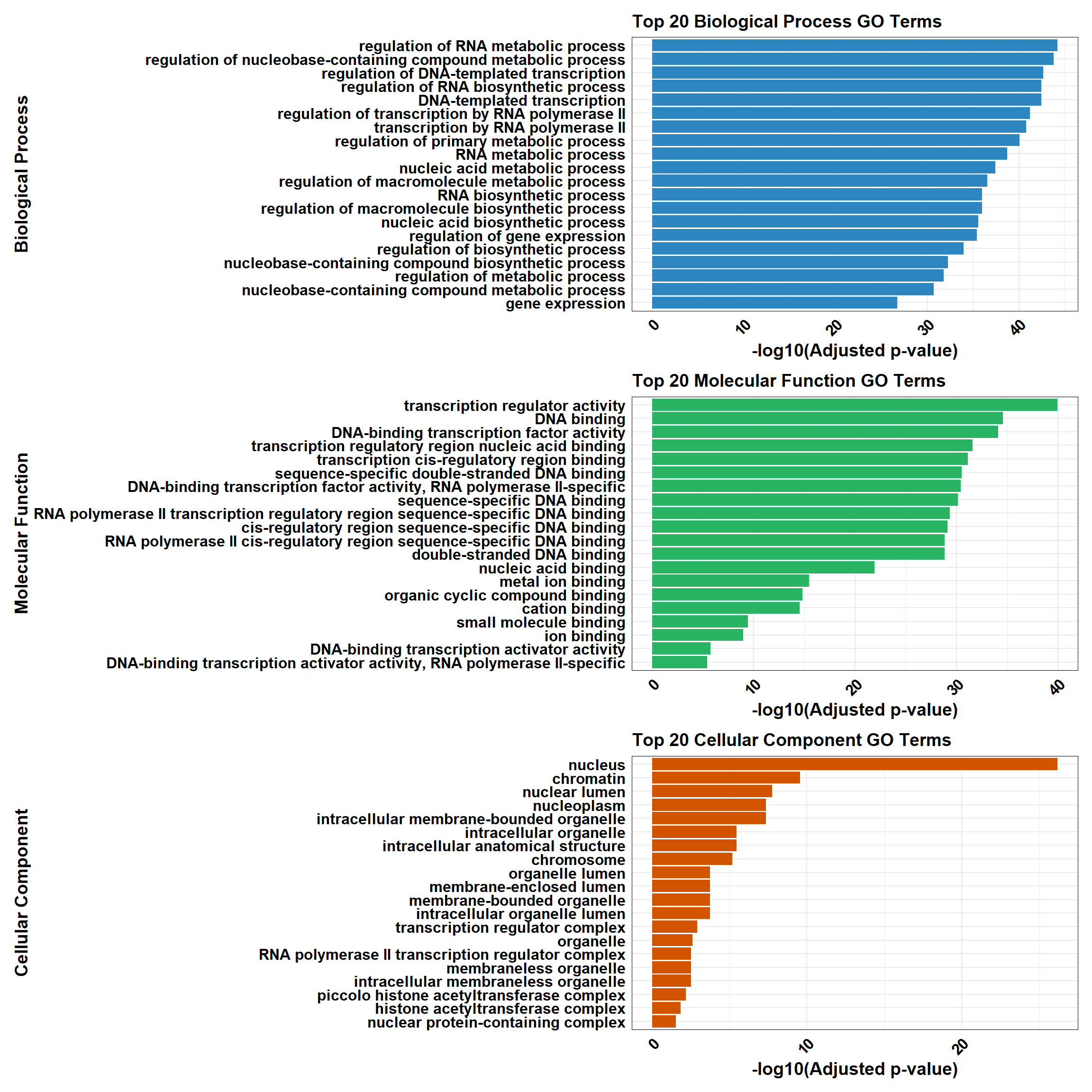
📌 DOX vs VEH (0.5 and 3hr) Pathway Enrichment
# Load required libraries
library(clusterProfiler)
library(org.Hs.eg.db) # Required for enrichPathway
library(gprofiler2)
library(ggplot2)
library(dplyr)
library(patchwork)
library(ReactomePA)

# Function for ClusterProfiler Reactome & KEGG Analysis
process_clusterProfiler <- function(gene_set, background, category, color, y_title) {
  # Perform enrichment based on the selected category
  if (category == "Reactome") {
    enrichment <- enrichPathway(
      gene = gene_set,
      organism = "human",
      pvalueCutoff = 0.05,
      pAdjustMethod = "BH",
      universe = background
    )
  } else if (category == "KEGG") {
    enrichment <- enrichKEGG(
      gene = gene_set,
      organism = "hsa",
      pvalueCutoff = 0.05,
      pAdjustMethod = "BH",
      universe = background
    )
  }

  # Check if enrichment results exist
  if (is.null(enrichment) || nrow(as.data.frame(enrichment)) == 0) {
    message(paste("No significant enrichment found for", category, "in ClusterProfiler"))
    return(NULL)
  }

  # Convert results to tibble and process top 20 terms
  enrichment_tibble <- as_tibble(as.data.frame(enrichment)) %>%
    mutate(Category = category,
           neglog = -log10(p.adjust)) %>%  # Compute -log10(p.adjust)
    arrange(desc(neglog)) %>%
    slice_head(n = min(20, nrow(.)))  # Ensure safe slicing

  # Generate plot
  plot <- ggplot(enrichment_tibble, aes(x = neglog, y = reorder(Description, neglog))) +
    geom_bar(stat = "identity", fill = color) +
    labs(x = "-log10(Adjusted p-value)",
         y = y_title,
         title = paste("Enriched", category, "Pathways")) +
    theme_minimal() +
    theme(
      axis.text.x = element_text(size = 12, face = "bold", colour = "black", angle = 45, hjust = 1),
      axis.text.y = element_text(size = 12, face = "bold", colour = "black"),
      axis.title.x = element_text(size = 14, face = "bold", colour = "black"),
      axis.title.y = element_text(size = 14, face = "bold", colour = "black"),
      plot.title = element_text(size = 14, face = "bold", colour = "black")
    )

  return(plot)
}

# Function for gProfiler Reactome & KEGG Analysis
process_gprofiler <- function(gene_set, background, category, color, y_title) {
  # Perform enrichment using gprofiler2
  enrichment <- gost(
    query = gene_set,
    organism = "hsapiens",
    user_threshold = 0.05,
    correction_method = "fdr",
    domain_scope = "custom",
    custom_bg = background,
    sources = category # Either "REAC" or "KEGG"
  )

  # Check if enrichment results exist
  if (is.null(enrichment$result) || nrow(enrichment$result) == 0) {
    message(paste("No significant enrichment found for", category, "in gProfiler"))
    return(NULL)
  }

  # Convert results to tibble and process top 20 terms
  enrichment_tibble <- enrichment$result %>%
    as_tibble() %>%
    mutate(Category = category,
           neglog = -log10(p_value)) %>%  # Compute -log10(p-value)
    arrange(desc(neglog)) %>%
    slice_head(n = min(20, nrow(.)))  # Ensure safe slicing

  # Generate plot
  plot <- ggplot(enrichment_tibble, aes(x = neglog, y = reorder(term_name, neglog))) +
    geom_bar(stat = "identity", fill = color) +
    labs(x = "-log10(p-value)",
         y = y_title,
         title = paste("Enriched", category, "Pathways")) +
    theme_minimal() +
    theme(
      axis.text.x = element_text(size = 12, face = "bold", colour = "black", angle = 45, hjust = 1),
      axis.text.y = element_text(size = 12, face = "bold", colour = "black"),
      axis.title.x = element_text(size = 14, face = "bold", colour = "black"),
      axis.title.y = element_text(size = 14, face = "bold", colour = "black"),
      plot.title = element_text(size = 14, face = "bold", colour = "black")
    )

  return(plot)
}

# Perform analysis for Reactome and KEGG using ClusterProfiler
cluster_reactome <- process_clusterProfiler(
  gene_set = DEG10,
  background = background,
  category = "Reactome",
  color = "#2E86C1",
  y_title = "Reactome Pathways"
)

cluster_kegg <- process_clusterProfiler(
  gene_set = DEG10,
  background = background,
  category = "KEGG",
  color = "#28B463",
  y_title = "KEGG Pathways"
)

# Combine Reactome and KEGG for ClusterProfiler
if (!is.null(cluster_reactome) && !is.null(cluster_kegg)) {
  cluster_combined <- cluster_reactome / cluster_kegg
} else if (!is.null(cluster_reactome)) {
  cluster_combined <- cluster_reactome
} else if (!is.null(cluster_kegg)) {
  cluster_combined <- cluster_kegg
} else {
  cluster_combined <- NULL
}

# Perform analysis for Reactome and KEGG using GProfiler
gprofiler_reactome <- process_gprofiler(
  gene_set = DEG10,
  background = background,
  category = "REAC",  # Corrected category for Reactome in gProfiler
  color = "#D35400",
  y_title = "Reactome Pathways"
)

gprofiler_kegg <- process_gprofiler(
  gene_set = DEG10,
  background = background,
  category = "KEGG",
  color = "#F39C12",
  y_title = "KEGG Pathways"
)

# Combine Reactome and KEGG for GProfiler
if (!is.null(gprofiler_reactome) && !is.null(gprofiler_kegg)) {
  gprofiler_combined <- gprofiler_reactome / gprofiler_kegg
} else if (!is.null(gprofiler_reactome)) {
  gprofiler_combined <- gprofiler_reactome
} else if (!is.null(gprofiler_kegg)) {
  gprofiler_combined <- gprofiler_kegg
} else {
  gprofiler_combined <- NULL
}

# Display plots (if they are not NULL)
if (!is.null(cluster_combined)) print(cluster_combined)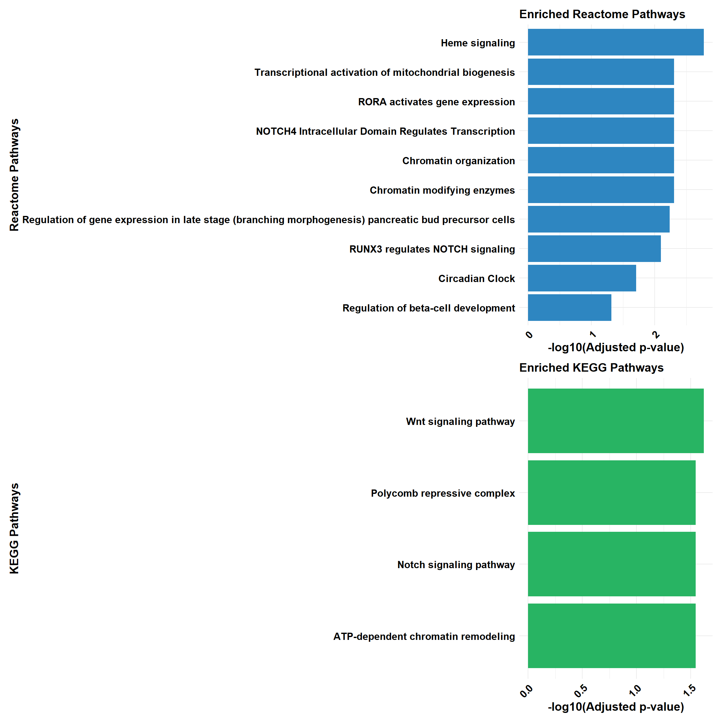
if (!is.null(gprofiler_combined)) print(gprofiler_combined)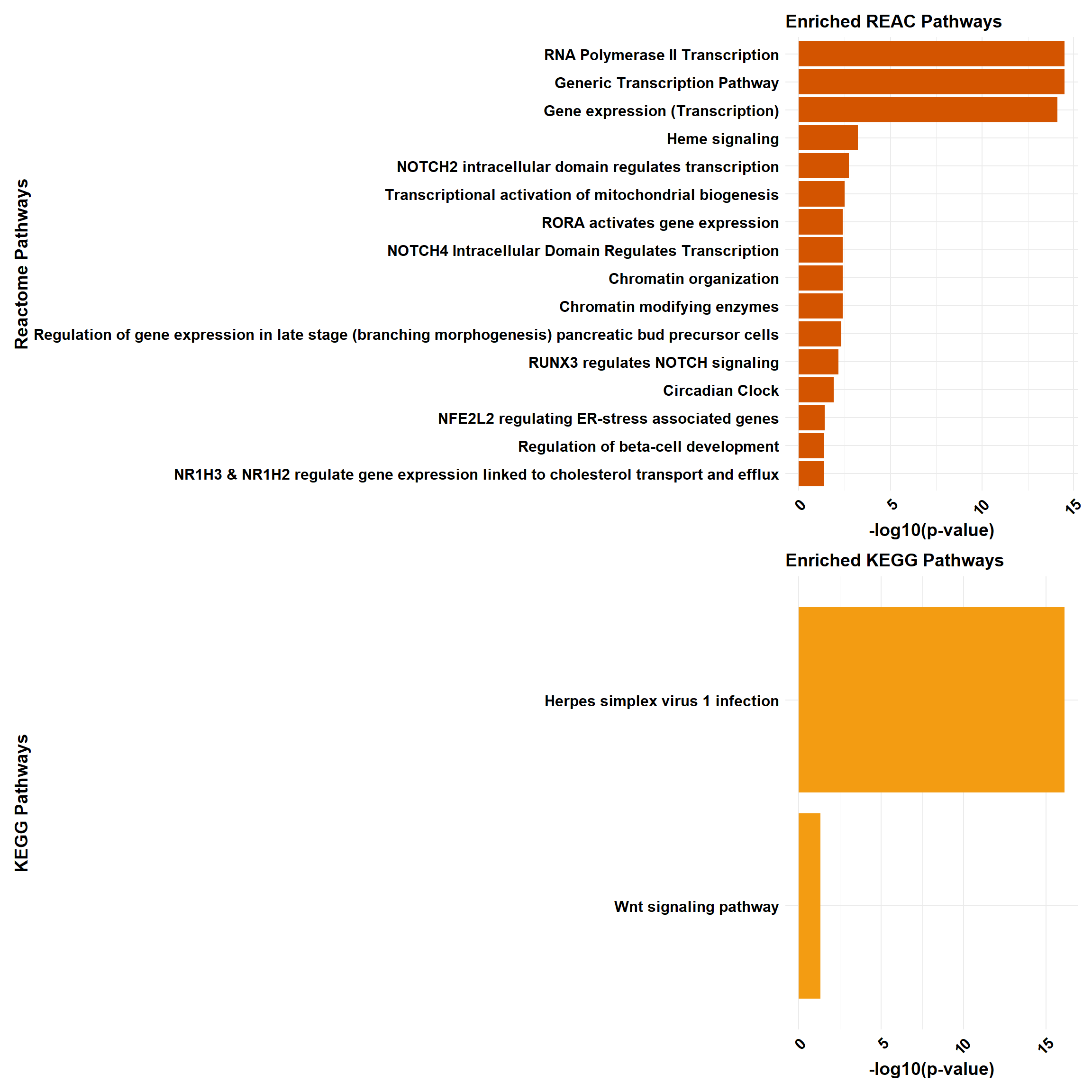
📌 DOX vs VEH (0.5 and 24hr)
📌 DOX vs VEH (0.5 and 24hr) GO Enrichment Clusterprofiler
# Perform GO enrichment analysis for BP, MF, and CC
go_enrichment_BP <- enrichGO(gene = DEG11,
                             OrgDb = org.Hs.eg.db,
                             keyType = "ENTREZID",
                             universe = background,
                             ont = "BP",
                             pvalueCutoff = 0.05)

go_enrichment_MF <- enrichGO(gene = DEG11,
                             OrgDb = org.Hs.eg.db,
                             keyType = "ENTREZID",
                             universe = background,
                             ont = "MF",
                             pvalueCutoff = 0.05)

go_enrichment_CC <- enrichGO(gene = DEG11,
                             OrgDb = org.Hs.eg.db,
                             keyType = "ENTREZID",
                             universe = background,
                             ont = "CC",
                             pvalueCutoff = 0.05)

# Convert each enrichment result to a tibble, add a category column, and select top 20 terms
process_enrichment_tibble <- function(enrichment, category) {
  if (is.null(enrichment) || nrow(as.data.frame(enrichment)) == 0) {
    return(tibble(Description = "No enriched terms", neglog = 0, Category = category))
  } else {
    enrichment %>%
      as_tibble() %>%
      mutate(Category = category,
             neglog = -log(p.adjust)) %>% # Add -log(p.adjust) column
      arrange(desc(neglog)) %>%          # Sort by -log(p.adjust)
      slice(1:20)                        # Select top 20 terms
  }
}

BP_Tibble <- process_enrichment_tibble(go_enrichment_BP, "Biological Process")
MF_Tibble <- process_enrichment_tibble(go_enrichment_MF, "Molecular Function")
CC_Tibble <- process_enrichment_tibble(go_enrichment_CC, "Cellular Component")

# Combine all tibbles
combined_GO_Tibble <- bind_rows(BP_Tibble, MF_Tibble, CC_Tibble)
# Function to generate enrichment plots
process_enrichment_plot <- function(tibble, title, color) {
  ggplot(data = tibble, aes(x = neglog, y = reorder(Description, neglog))) +
    geom_bar(stat = "identity", fill = color) +
    labs(x = "-log(p-adjust)",
         y = title,
         title = paste("Top 20", title, "GO Terms")) +
    theme_minimal() +
    theme(
      axis.text.x = element_text(size = 12, face = "bold", colour = "black", angle = 45, hjust = 1),
      axis.text.y = element_text(size = 12, face = "bold", colour = "black"),
      axis.title.x = element_text(size = 14, face = "bold", colour = "black"),
      axis.title.y = element_text(size = 14, face = "bold", colour = "black"),
      plot.title = element_text(size = 14, face = "bold", colour = "black"),
      panel.border = element_rect(colour = "black", fill = NA, size = 0.3)
    ) +
    xlim(c(0, max(tibble$neglog) + 1))
}

# Generate separate plots
plot_BP <- process_enrichment_plot(BP_Tibble, "Biological Process", "#2E86C1")
plot_MF <- process_enrichment_plot(MF_Tibble, "Molecular Function", "#28B463")
plot_CC <- process_enrichment_plot(CC_Tibble, "Cellular Component", "#D35400")

# Combine the plots using patchwork
combined_plot <- plot_BP / plot_MF / plot_CC

# Display the combined plot
combined_plot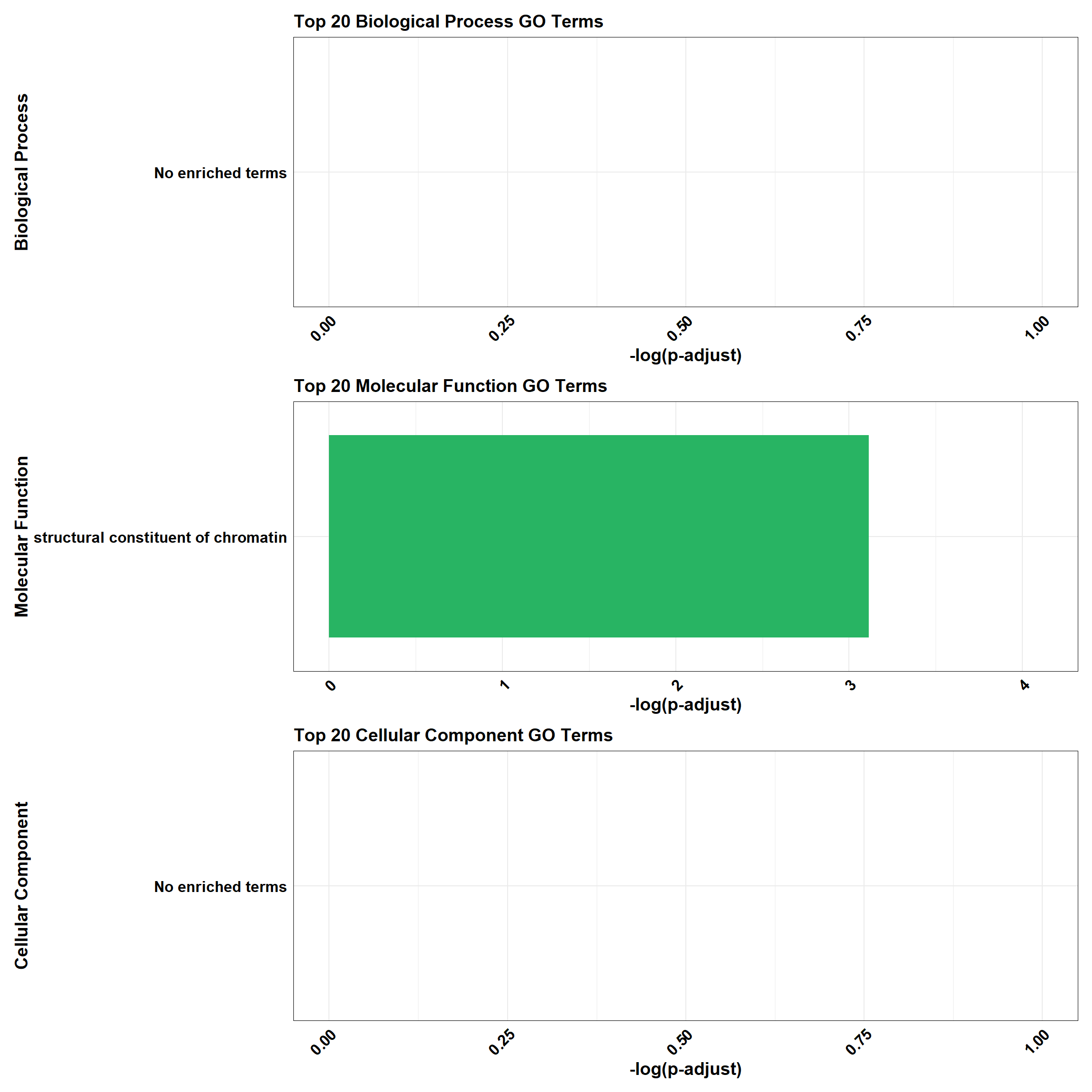
| Version | Author | Date |
|---|---|---|
| f57065b | sayanpaul01 | 2025-02-20 |
📌 DOX vs VEH (0.5 and 24hr) GO Enrichment g:Profiler
# Load the gprofiler2 package
library(gprofiler2)
library(ggplot2)
library(dplyr)
library(patchwork)

# Perform GO enrichment analysis with gprofiler2
gost_results <- gost(
  query = DEG11,
  organism = "hsapiens",   # Human organism
  user_threshold = 0.05,   # Adjusted p-value cutoff
  correction_method = "fdr", # Multiple testing correction
  domain_scope = "custom", # Use custom background
  custom_bg = background,    # Background set of genes
  sources = c("GO:BP", "GO:MF", "GO:CC") # Analyze GO categories
)

# Check if enrichment results exist
if (is.null(gost_results$result) || nrow(gost_results$result) == 0) {
  # If no enriched terms, create a placeholder dataframe
  combined_results <- tibble(
    term_name = "No enriched terms",
    p.adjust = NA,
    source = "N/A",
    Category = "N/A"
  )
} else {
  # Convert results to a data frame
  gost_results_df <- gost_results$result

  # Add a column for adjusted p-value
  gost_results_df <- gost_results_df %>%
    rename(p.adjust = p_value)

  # Separate results for BP, MF, and CC
  BP_results <- gost_results_df %>%
    filter(source == "GO:BP") %>%
    mutate(Category = "Biological Process")

  MF_results <- gost_results_df %>%
    filter(source == "GO:MF") %>%
    mutate(Category = "Molecular Function")

  CC_results <- gost_results_df %>%
    filter(source == "GO:CC") %>%
    mutate(Category = "Cellular Component")

  # Select the top 20 terms by adjusted p-value for each category
  top_BP <- BP_results %>%
    arrange(p.adjust) %>%
    slice_head(n = 20)

  top_MF <- MF_results %>%
    arrange(p.adjust) %>%
    slice_head(n = 20)

  top_CC <- CC_results %>%
    arrange(p.adjust) %>%
    slice_head(n = 20)

  # Combine all categories
  combined_results <- bind_rows(top_BP, top_MF, top_CC)
}

# Ensure all columns are atomic types for CSV export
combined_results_clean <- combined_results %>%
  mutate(across(everything(), ~ if (is.list(.)) sapply(., toString) else .))

# Function for plotting top terms
plot_gprofiler_results <- function(data, title, color) {
  ggplot(data, aes(x = -log10(p.adjust), y = reorder(term_name, -log10(p.adjust)))) +
    geom_bar(stat = "identity", fill = color) +
    labs(
      x = "-log10(Adjusted p-value)",
      y = title,
      title = paste("Top 20", title, "GO Terms")
    ) +
    theme_minimal() +
    theme(
      axis.text.x = element_text(size = 12, face = "bold", colour = "black", angle = 45, hjust = 1),
      axis.text.y = element_text(size = 12, face = "bold", colour = "black"),
      axis.title.x = element_text(size = 14, face = "bold", colour = "black"),
      axis.title.y = element_text(size = 14, face = "bold", colour = "black"),
      plot.title = element_text(size = 14, face = "bold", colour = "black"),
      panel.border = element_rect(colour = "black", fill = NA, size = 0.3)
    )
}

# Check if there are enrichment terms to plot
if (nrow(combined_results) == 1 && combined_results$term_name == "No enriched terms") {
  message("No enriched GO terms found for the input gene set.")
} else {
  # Plot the top 20 terms for each category
  plot_BP <- plot_gprofiler_results(top_BP, "Biological Process", "#2E86C1")
  plot_MF <- plot_gprofiler_results(top_MF, "Molecular Function", "#28B463")
  plot_CC <- plot_gprofiler_results(top_CC, "Cellular Component", "#D35400")

  # Combine the plots using patchwork
  combined_plot <- plot_BP / plot_MF / plot_CC

  # Display the combined plot
  combined_plot
}
📌 DOX vs VEH (0.5 and 24hr) Pathway Enrichment
# Load required libraries
library(clusterProfiler)
library(org.Hs.eg.db) # Required for enrichPathway
library(gprofiler2)
library(ggplot2)
library(dplyr)
library(patchwork)
library(ReactomePA)

# Function for ClusterProfiler Reactome & KEGG Analysis
process_clusterProfiler <- function(gene_set, background, category, color, y_title) {
  # Perform enrichment based on the selected category
  if (category == "Reactome") {
    enrichment <- enrichPathway(
      gene = gene_set,
      organism = "human",
      pvalueCutoff = 0.05,
      pAdjustMethod = "BH",
      universe = background
    )
  } else if (category == "KEGG") {
    enrichment <- enrichKEGG(
      gene = gene_set,
      organism = "hsa",
      pvalueCutoff = 0.05,
      pAdjustMethod = "BH",
      universe = background
    )
  }

  # Check if enrichment results exist
  if (is.null(enrichment) || nrow(as.data.frame(enrichment)) == 0) {
    message(paste("No significant enrichment found for", category, "in ClusterProfiler"))
    return(NULL)
  }

  # Convert results to tibble and process top 20 terms
  enrichment_tibble <- as_tibble(as.data.frame(enrichment)) %>%
    mutate(Category = category,
           neglog = -log10(p.adjust)) %>%  # Compute -log10(p.adjust)
    arrange(desc(neglog)) %>%
    slice_head(n = min(20, nrow(.)))  # Ensure safe slicing

  # Generate plot
  plot <- ggplot(enrichment_tibble, aes(x = neglog, y = reorder(Description, neglog))) +
    geom_bar(stat = "identity", fill = color) +
    labs(x = "-log10(Adjusted p-value)",
         y = y_title,
         title = paste("Enriched", category, "Pathways")) +
    theme_minimal() +
    theme(
      axis.text.x = element_text(size = 12, face = "bold", colour = "black", angle = 45, hjust = 1),
      axis.text.y = element_text(size = 12, face = "bold", colour = "black"),
      axis.title.x = element_text(size = 14, face = "bold", colour = "black"),
      axis.title.y = element_text(size = 14, face = "bold", colour = "black"),
      plot.title = element_text(size = 14, face = "bold", colour = "black")
    )

  return(plot)
}

# Function for gProfiler Reactome & KEGG Analysis
process_gprofiler <- function(gene_set, background, category, color, y_title) {
  # Perform enrichment using gprofiler2
  enrichment <- gost(
    query = gene_set,
    organism = "hsapiens",
    user_threshold = 0.05,
    correction_method = "fdr",
    domain_scope = "custom",
    custom_bg = background,
    sources = category # Either "REAC" or "KEGG"
  )

  # Check if enrichment results exist
  if (is.null(enrichment$result) || nrow(enrichment$result) == 0) {
    message(paste("No significant enrichment found for", category, "in gProfiler"))
    return(NULL)
  }

  # Convert results to tibble and process top 20 terms
  enrichment_tibble <- enrichment$result %>%
    as_tibble() %>%
    mutate(Category = category,
           neglog = -log10(p_value)) %>%  # Compute -log10(p-value)
    arrange(desc(neglog)) %>%
    slice_head(n = min(20, nrow(.)))  # Ensure safe slicing

  # Generate plot
  plot <- ggplot(enrichment_tibble, aes(x = neglog, y = reorder(term_name, neglog))) +
    geom_bar(stat = "identity", fill = color) +
    labs(x = "-log10(p-value)",
         y = y_title,
         title = paste("Enriched", category, "Pathways")) +
    theme_minimal() +
    theme(
      axis.text.x = element_text(size = 12, face = "bold", colour = "black", angle = 45, hjust = 1),
      axis.text.y = element_text(size = 12, face = "bold", colour = "black"),
      axis.title.x = element_text(size = 14, face = "bold", colour = "black"),
      axis.title.y = element_text(size = 14, face = "bold", colour = "black"),
      plot.title = element_text(size = 14, face = "bold", colour = "black")
    )

  return(plot)
}

# Perform analysis for Reactome and KEGG using ClusterProfiler
cluster_reactome <- process_clusterProfiler(
  gene_set = DEG11,
  background = background,
  category = "Reactome",
  color = "#2E86C1",
  y_title = "Reactome Pathways"
)

cluster_kegg <- process_clusterProfiler(
  gene_set = DEG11,
  background = background,
  category = "KEGG",
  color = "#28B463",
  y_title = "KEGG Pathways"
)

# Combine Reactome and KEGG for ClusterProfiler
if (!is.null(cluster_reactome) && !is.null(cluster_kegg)) {
  cluster_combined <- cluster_reactome / cluster_kegg
} else if (!is.null(cluster_reactome)) {
  cluster_combined <- cluster_reactome
} else if (!is.null(cluster_kegg)) {
  cluster_combined <- cluster_kegg
} else {
  cluster_combined <- NULL
}

# Perform analysis for Reactome and KEGG using GProfiler
gprofiler_reactome <- process_gprofiler(
  gene_set = DEG11,
  background = background,
  category = "REAC",  # Corrected category for Reactome in gProfiler
  color = "#D35400",
  y_title = "Reactome Pathways"
)

gprofiler_kegg <- process_gprofiler(
  gene_set = DEG11,
  background = background,
  category = "KEGG",
  color = "#F39C12",
  y_title = "KEGG Pathways"
)

# Combine Reactome and KEGG for GProfiler
if (!is.null(gprofiler_reactome) && !is.null(gprofiler_kegg)) {
  gprofiler_combined <- gprofiler_reactome / gprofiler_kegg
} else if (!is.null(gprofiler_reactome)) {
  gprofiler_combined <- gprofiler_reactome
} else if (!is.null(gprofiler_kegg)) {
  gprofiler_combined <- gprofiler_kegg
} else {
  gprofiler_combined <- NULL
}

# Display plots (if they are not NULL)
if (!is.null(cluster_combined)) print(cluster_combined)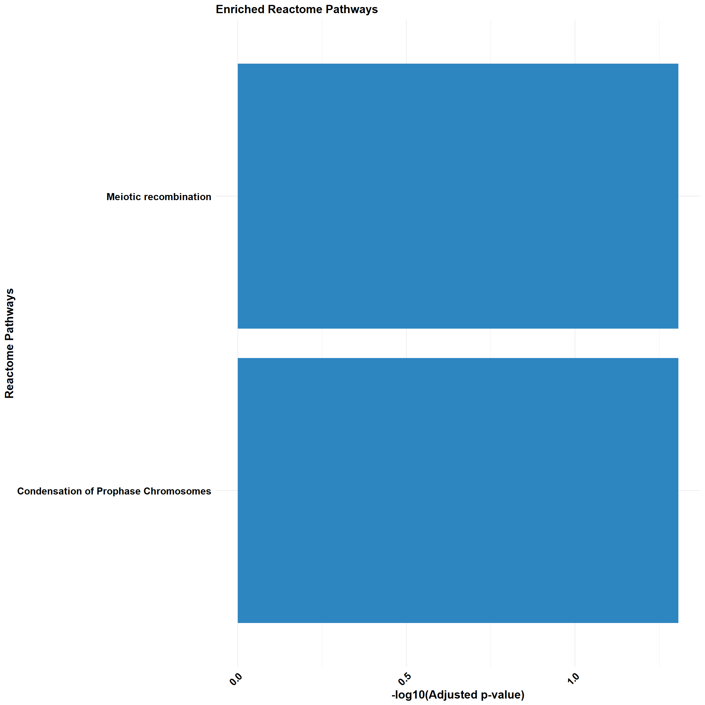
if (!is.null(gprofiler_combined)) print(gprofiler_combined)📌 DOX vs VEH (0.5 and 48hr)
📌 DOX vs VEH (0.5 and 48hr) GO Enrichment Clusterprofiler
# Perform GO enrichment analysis for BP, MF, and CC
go_enrichment_BP <- enrichGO(gene = DEG12,
                             OrgDb = org.Hs.eg.db,
                             keyType = "ENTREZID",
                             universe = background,
                             ont = "BP",
                             pvalueCutoff = 0.05)

go_enrichment_MF <- enrichGO(gene = DEG12,
                             OrgDb = org.Hs.eg.db,
                             keyType = "ENTREZID",
                             universe = background,
                             ont = "MF",
                             pvalueCutoff = 0.05)

go_enrichment_CC <- enrichGO(gene = DEG12,
                             OrgDb = org.Hs.eg.db,
                             keyType = "ENTREZID",
                             universe = background,
                             ont = "CC",
                             pvalueCutoff = 0.05)

# Convert each enrichment result to a tibble, add a category column, and select top 20 terms
process_enrichment_tibble <- function(enrichment, category) {
  if (is.null(enrichment) || nrow(as.data.frame(enrichment)) == 0) {
    return(tibble(Description = "No enriched terms", neglog = 0, Category = category))
  } else {
    enrichment %>%
      as_tibble() %>%
      mutate(Category = category,
             neglog = -log(p.adjust)) %>% # Add -log(p.adjust) column
      arrange(desc(neglog)) %>%          # Sort by -log(p.adjust)
      slice(1:20)                        # Select top 20 terms
  }
}

BP_Tibble <- process_enrichment_tibble(go_enrichment_BP, "Biological Process")
MF_Tibble <- process_enrichment_tibble(go_enrichment_MF, "Molecular Function")
CC_Tibble <- process_enrichment_tibble(go_enrichment_CC, "Cellular Component")

# Combine all tibbles
combined_GO_Tibble <- bind_rows(BP_Tibble, MF_Tibble, CC_Tibble)
# Function to generate enrichment plots
process_enrichment_plot <- function(tibble, title, color) {
  ggplot(data = tibble, aes(x = neglog, y = reorder(Description, neglog))) +
    geom_bar(stat = "identity", fill = color) +
    labs(x = "-log(p-adjust)",
         y = title,
         title = paste("Top 20", title, "GO Terms")) +
    theme_minimal() +
    theme(
      axis.text.x = element_text(size = 12, face = "bold", colour = "black", angle = 45, hjust = 1),
      axis.text.y = element_text(size = 12, face = "bold", colour = "black"),
      axis.title.x = element_text(size = 14, face = "bold", colour = "black"),
      axis.title.y = element_text(size = 14, face = "bold", colour = "black"),
      plot.title = element_text(size = 14, face = "bold", colour = "black"),
      panel.border = element_rect(colour = "black", fill = NA, size = 0.3)
    ) +
    xlim(c(0, max(tibble$neglog) + 1))
}

# Generate separate plots
plot_BP <- process_enrichment_plot(BP_Tibble, "Biological Process", "#2E86C1")
plot_MF <- process_enrichment_plot(MF_Tibble, "Molecular Function", "#28B463")
plot_CC <- process_enrichment_plot(CC_Tibble, "Cellular Component", "#D35400")

# Combine the plots using patchwork
combined_plot <- plot_BP / plot_MF / plot_CC

# Display the combined plot
combined_plot
| Version | Author | Date |
|---|---|---|
| f57065b | sayanpaul01 | 2025-02-20 |
📌 DOX vs VEH (0.5 and 48hr) GO Enrichment g:Profiler
# Load the gprofiler2 package
library(gprofiler2)
library(ggplot2)
library(dplyr)
library(patchwork)

# Perform GO enrichment analysis with gprofiler2
gost_results <- gost(
  query = DEG12,
  organism = "hsapiens",   # Human organism
  user_threshold = 0.05,   # Adjusted p-value cutoff
  correction_method = "fdr", # Multiple testing correction
  domain_scope = "custom", # Use custom background
  custom_bg = background,    # Background set of genes
  sources = c("GO:BP", "GO:MF", "GO:CC") # Analyze GO categories
)

# Check if enrichment results exist
if (is.null(gost_results$result) || nrow(gost_results$result) == 0) {
  # If no enriched terms, create a placeholder dataframe
  combined_results <- tibble(
    term_name = "No enriched terms",
    p.adjust = NA,
    source = "N/A",
    Category = "N/A"
  )
} else {
  # Convert results to a data frame
  gost_results_df <- gost_results$result

  # Add a column for adjusted p-value
  gost_results_df <- gost_results_df %>%
    rename(p.adjust = p_value)

  # Separate results for BP, MF, and CC
  BP_results <- gost_results_df %>%
    filter(source == "GO:BP") %>%
    mutate(Category = "Biological Process")

  MF_results <- gost_results_df %>%
    filter(source == "GO:MF") %>%
    mutate(Category = "Molecular Function")

  CC_results <- gost_results_df %>%
    filter(source == "GO:CC") %>%
    mutate(Category = "Cellular Component")

  # Select the top 20 terms by adjusted p-value for each category
  top_BP <- BP_results %>%
    arrange(p.adjust) %>%
    slice_head(n = 20)

  top_MF <- MF_results %>%
    arrange(p.adjust) %>%
    slice_head(n = 20)

  top_CC <- CC_results %>%
    arrange(p.adjust) %>%
    slice_head(n = 20)

  # Combine all categories
  combined_results <- bind_rows(top_BP, top_MF, top_CC)
}

# Ensure all columns are atomic types for CSV export
combined_results_clean <- combined_results %>%
  mutate(across(everything(), ~ if (is.list(.)) sapply(., toString) else .))

# Function for plotting top terms
plot_gprofiler_results <- function(data, title, color) {
  ggplot(data, aes(x = -log10(p.adjust), y = reorder(term_name, -log10(p.adjust)))) +
    geom_bar(stat = "identity", fill = color) +
    labs(
      x = "-log10(Adjusted p-value)",
      y = title,
      title = paste("Top 20", title, "GO Terms")
    ) +
    theme_minimal() +
    theme(
      axis.text.x = element_text(size = 12, face = "bold", colour = "black", angle = 45, hjust = 1),
      axis.text.y = element_text(size = 12, face = "bold", colour = "black"),
      axis.title.x = element_text(size = 14, face = "bold", colour = "black"),
      axis.title.y = element_text(size = 14, face = "bold", colour = "black"),
      plot.title = element_text(size = 14, face = "bold", colour = "black"),
      panel.border = element_rect(colour = "black", fill = NA, size = 0.3)
    )
}

# Check if there are enrichment terms to plot
if (nrow(combined_results) == 1 && combined_results$term_name == "No enriched terms") {
  message("No enriched GO terms found for the input gene set.")
} else {
  # Plot the top 20 terms for each category
  plot_BP <- plot_gprofiler_results(top_BP, "Biological Process", "#2E86C1")
  plot_MF <- plot_gprofiler_results(top_MF, "Molecular Function", "#28B463")
  plot_CC <- plot_gprofiler_results(top_CC, "Cellular Component", "#D35400")

  # Combine the plots using patchwork
  combined_plot <- plot_BP / plot_MF / plot_CC

  # Display the combined plot
  combined_plot
}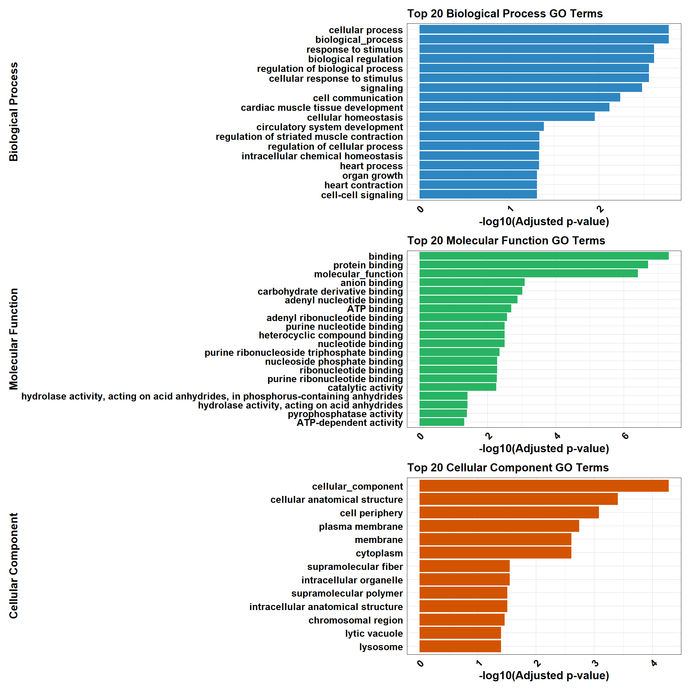
📌 DOX vs VEH (0.5 and 48hr) Pathway Enrichment
# Load required libraries
library(clusterProfiler)
library(org.Hs.eg.db) # Required for enrichPathway
library(gprofiler2)
library(ggplot2)
library(dplyr)
library(patchwork)
library(ReactomePA)

# Function for ClusterProfiler Reactome & KEGG Analysis
process_clusterProfiler <- function(gene_set, background, category, color, y_title) {
  # Perform enrichment based on the selected category
  if (category == "Reactome") {
    enrichment <- enrichPathway(
      gene = gene_set,
      organism = "human",
      pvalueCutoff = 0.05,
      pAdjustMethod = "BH",
      universe = background
    )
  } else if (category == "KEGG") {
    enrichment <- enrichKEGG(
      gene = gene_set,
      organism = "hsa",
      pvalueCutoff = 0.05,
      pAdjustMethod = "BH",
      universe = background
    )
  }

  # Check if enrichment results exist
  if (is.null(enrichment) || nrow(as.data.frame(enrichment)) == 0) {
    message(paste("No significant enrichment found for", category, "in ClusterProfiler"))
    return(NULL)
  }

  # Convert results to tibble and process top 20 terms
  enrichment_tibble <- as_tibble(as.data.frame(enrichment)) %>%
    mutate(Category = category,
           neglog = -log10(p.adjust)) %>%  # Compute -log10(p.adjust)
    arrange(desc(neglog)) %>%
    slice_head(n = min(20, nrow(.)))  # Ensure safe slicing

  # Generate plot
  plot <- ggplot(enrichment_tibble, aes(x = neglog, y = reorder(Description, neglog))) +
    geom_bar(stat = "identity", fill = color) +
    labs(x = "-log10(Adjusted p-value)",
         y = y_title,
         title = paste("Enriched", category, "Pathways")) +
    theme_minimal() +
    theme(
      axis.text.x = element_text(size = 12, face = "bold", colour = "black", angle = 45, hjust = 1),
      axis.text.y = element_text(size = 12, face = "bold", colour = "black"),
      axis.title.x = element_text(size = 14, face = "bold", colour = "black"),
      axis.title.y = element_text(size = 14, face = "bold", colour = "black"),
      plot.title = element_text(size = 14, face = "bold", colour = "black")
    )

  return(plot)
}

# Function for gProfiler Reactome & KEGG Analysis
process_gprofiler <- function(gene_set, background, category, color, y_title) {
  # Perform enrichment using gprofiler2
  enrichment <- gost(
    query = gene_set,
    organism = "hsapiens",
    user_threshold = 0.05,
    correction_method = "fdr",
    domain_scope = "custom",
    custom_bg = background,
    sources = category # Either "REAC" or "KEGG"
  )

  # Check if enrichment results exist
  if (is.null(enrichment$result) || nrow(enrichment$result) == 0) {
    message(paste("No significant enrichment found for", category, "in gProfiler"))
    return(NULL)
  }

  # Convert results to tibble and process top 20 terms
  enrichment_tibble <- enrichment$result %>%
    as_tibble() %>%
    mutate(Category = category,
           neglog = -log10(p_value)) %>%  # Compute -log10(p-value)
    arrange(desc(neglog)) %>%
    slice_head(n = min(20, nrow(.)))  # Ensure safe slicing

  # Generate plot
  plot <- ggplot(enrichment_tibble, aes(x = neglog, y = reorder(term_name, neglog))) +
    geom_bar(stat = "identity", fill = color) +
    labs(x = "-log10(p-value)",
         y = y_title,
         title = paste("Enriched", category, "Pathways")) +
    theme_minimal() +
    theme(
      axis.text.x = element_text(size = 12, face = "bold", colour = "black", angle = 45, hjust = 1),
      axis.text.y = element_text(size = 12, face = "bold", colour = "black"),
      axis.title.x = element_text(size = 14, face = "bold", colour = "black"),
      axis.title.y = element_text(size = 14, face = "bold", colour = "black"),
      plot.title = element_text(size = 14, face = "bold", colour = "black")
    )

  return(plot)
}

# Perform analysis for Reactome and KEGG using ClusterProfiler
cluster_reactome <- process_clusterProfiler(
  gene_set = DEG12,
  background = background,
  category = "Reactome",
  color = "#2E86C1",
  y_title = "Reactome Pathways"
)

cluster_kegg <- process_clusterProfiler(
  gene_set = DEG12,
  background = background,
  category = "KEGG",
  color = "#28B463",
  y_title = "KEGG Pathways"
)

# Combine Reactome and KEGG for ClusterProfiler
if (!is.null(cluster_reactome) && !is.null(cluster_kegg)) {
  cluster_combined <- cluster_reactome / cluster_kegg
} else if (!is.null(cluster_reactome)) {
  cluster_combined <- cluster_reactome
} else if (!is.null(cluster_kegg)) {
  cluster_combined <- cluster_kegg
} else {
  cluster_combined <- NULL
}

# Perform analysis for Reactome and KEGG using GProfiler
gprofiler_reactome <- process_gprofiler(
  gene_set = DEG12,
  background = background,
  category = "REAC",  # Corrected category for Reactome in gProfiler
  color = "#D35400",
  y_title = "Reactome Pathways"
)

gprofiler_kegg <- process_gprofiler(
  gene_set = DEG12,
  background = background,
  category = "KEGG",
  color = "#F39C12",
  y_title = "KEGG Pathways"
)

# Combine Reactome and KEGG for GProfiler
if (!is.null(gprofiler_reactome) && !is.null(gprofiler_kegg)) {
  gprofiler_combined <- gprofiler_reactome / gprofiler_kegg
} else if (!is.null(gprofiler_reactome)) {
  gprofiler_combined <- gprofiler_reactome
} else if (!is.null(gprofiler_kegg)) {
  gprofiler_combined <- gprofiler_kegg
} else {
  gprofiler_combined <- NULL
}

# Display plots (if they are not NULL)
if (!is.null(cluster_combined)) print(cluster_combined)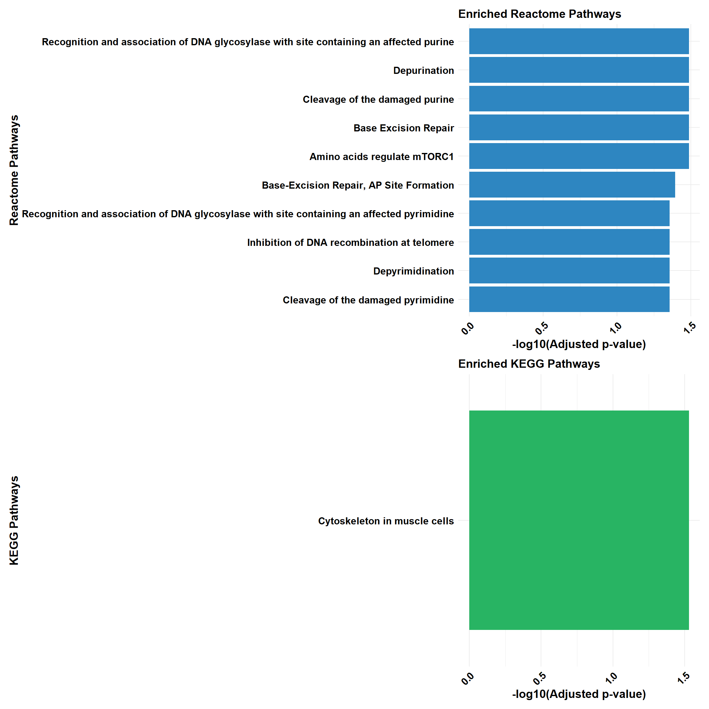
if (!is.null(gprofiler_combined)) print(gprofiler_combined)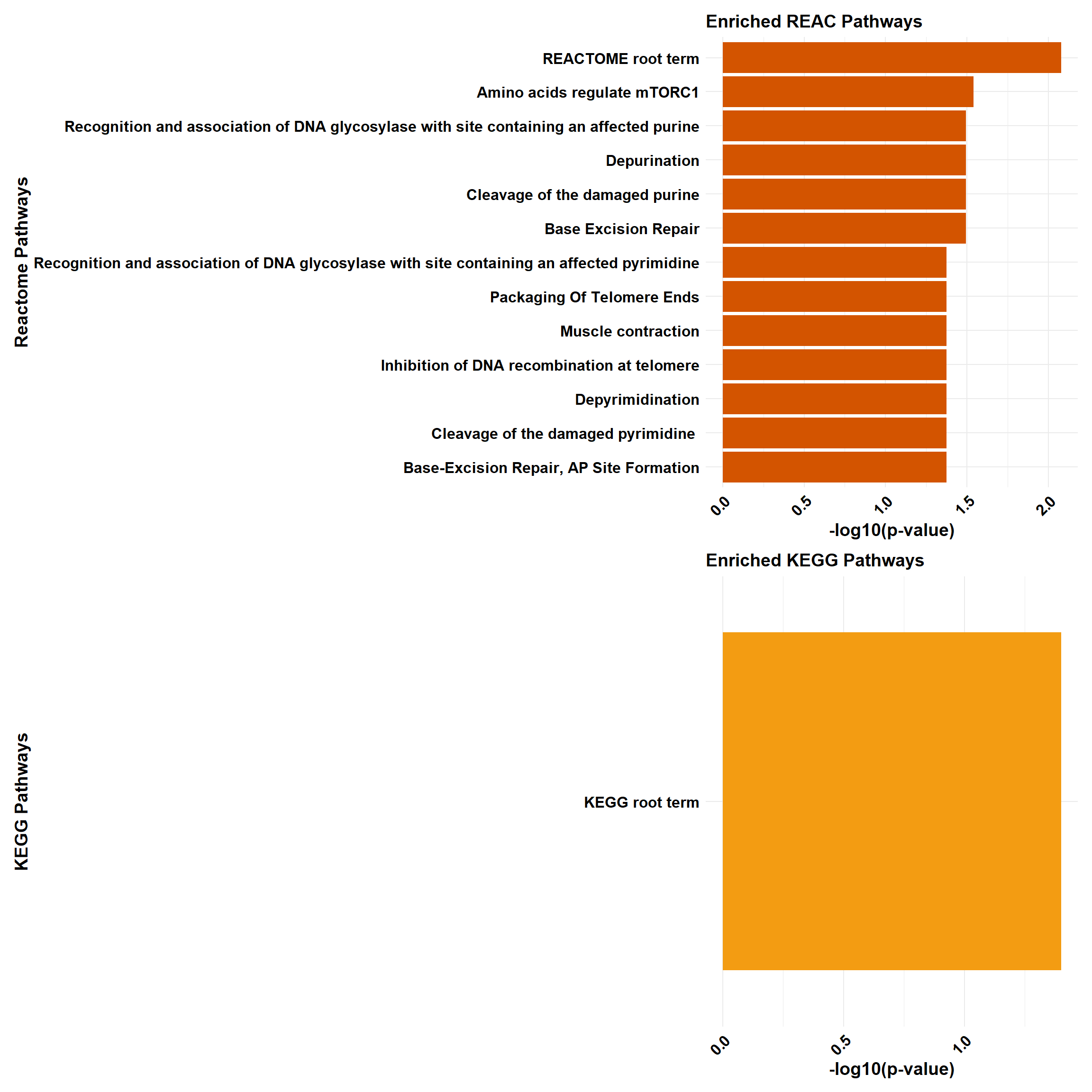
📌 Top BP (Cluster Profiler)
### Load Required Libraries
library(tidyverse)
library(ComplexHeatmap)
Warning: package 'ComplexHeatmap' was built under R version 4.3.1library(circlize)Warning: package 'circlize' was built under R version 4.3.3library(grid)
### Input GO Enrichment Files
go_files <- list(
"CX_0.1_3" = "data/BP/All_Terms/GO_BP_CX_0.1_3.csv",
"CX_0.1_24" = "data/BP/All_Terms/GO_BP_CX_0.1_24.csv",
"CX_0.1_48" = "data/BP/All_Terms/GO_BP_CX_0.1_48.csv",
"CX_0.5_3" = "data/BP/All_Terms/GO_BP_CX_0.5_3.csv",
"CX_0.5_24" = "data/BP/All_Terms/GO_BP_CX_0.5_24.csv",
"CX_0.5_48" = "data/BP/All_Terms/GO_BP_CX_0.5_48.csv",
"DOX_0.1_3" = "data/BP/All_Terms/GO_BP_DOX_0.1_3.csv",
"DOX_0.1_24"= "data/BP/All_Terms/GO_BP_DOX_0.1_24.csv",
"DOX_0.1_48"= "data/BP/All_Terms/GO_BP_DOX_0.1_48.csv",
"DOX_0.5_3" = "data/BP/All_Terms/GO_BP_DOX_0.5_3.csv",
"DOX_0.5_24"= "data/BP/All_Terms/GO_BP_DOX_0.5_24.csv",
"DOX_0.5_48"= "data/BP/All_Terms/GO_BP_DOX_0.5_48.csv"
)
### Step 1: Extract Top 5 GO Terms with Padj < 0.05
top_go_terms <- map(go_files, function(file) {
df <- tryCatch(read.csv(file), error = function(e) return(NULL))
if (!is.null(df) && nrow(df) > 0) {
df %>%
as_tibble() %>%
filter(p.adjust < 0.05) %>%
arrange(p.adjust) %>%
dplyr::select(Description) %>%
slice_head(n = 5) %>%
pull(Description) %>%
unique()
} else {
character(0)
}
}) %>% unlist() %>% unique()
### Step 2: Build Combined Table with P, P.adj, and -log10(p)
go_matrix_df <- map_dfr(names(go_files), function(cond) {
file <- go_files[[cond]]
df <- tryCatch(read.csv(file), error = function(e) return(data.frame()))
if (nrow(df) == 0) {
tibble(Description = top_go_terms, pvalue = NA, p.adjust = NA, log10p = NA, Condition = cond)
} else {
df %>%
as_tibble() %>%
dplyr::select(Description, pvalue, p.adjust) %>%
filter(Description %in% top_go_terms) %>%
mutate(log10p = -log10(pvalue)) %>%
right_join(tibble(Description = top_go_terms), by = "Description") %>%
mutate(Condition = cond)
}
})
### Step 3: Convert to Heatmap Matrices
heatmap_data <- go_matrix_df %>%
dplyr::select(Description, Condition, log10p) %>%
pivot_wider(names_from = Condition, values_from = log10p) %>%
column_to_rownames("Description") %>%
as.matrix()
pval_matrix <- go_matrix_df %>%
dplyr::select(Description, Condition, pvalue) %>%
pivot_wider(names_from = Condition, values_from = pvalue) %>%
column_to_rownames("Description") %>%
as.matrix()
p_adj_matrix <- go_matrix_df %>%
dplyr::select(Description, Condition, p.adjust) %>%
pivot_wider(names_from = Condition, values_from = p.adjust) %>%
column_to_rownames("Description") %>%
as.matrix()
### Step 4: Define Color Scale on Raw P-values
breaks <- seq(0, 20, by = 2.5)
palette <- colorRampPalette(c("white", "#fde0dd", "#fa9fb5", "#f768a1", "#c51b8a", "#7a0177", "#49006a"))(length(breaks))
col_fun <- colorRamp2(breaks, palette)
### Step 5: Plot Heatmap with Stars Based on Padj < 0.05
ht <- Heatmap(
heatmap_data,
name = "-log10(p)",
col = col_fun,
na_col = "white",
rect_gp = gpar(col = "black", lwd = 0.5),
cluster_rows = FALSE,
cluster_columns = FALSE,
row_names_gp = gpar(fontsize = 9),
column_names_gp = gpar(fontsize = 9),
column_names_rot = 45,
row_names_max_width = max_text_width(rownames(heatmap_data), gp = gpar(fontsize = 9)),
cell_fun = function(j, i, x, y, width, height, fill) {
if (!is.na(p_adj_matrix[i, j]) && p_adj_matrix[i, j] < 0.05) {
grid.text("*", x, y, gp = gpar(fontsize = 12))
}
},
heatmap_legend_param = list(
title = "-log10(p value)",
at = breaks,
labels = as.character(breaks),
legend_width = unit(5, "cm"),
direction = "horizontal",
title_gp = gpar(fontsize = 10, fontface = "bold"),
labels_gp = gpar(fontsize = 9)
)
)
### 🖼 Final Draw
draw(ht, heatmap_legend_side = "top")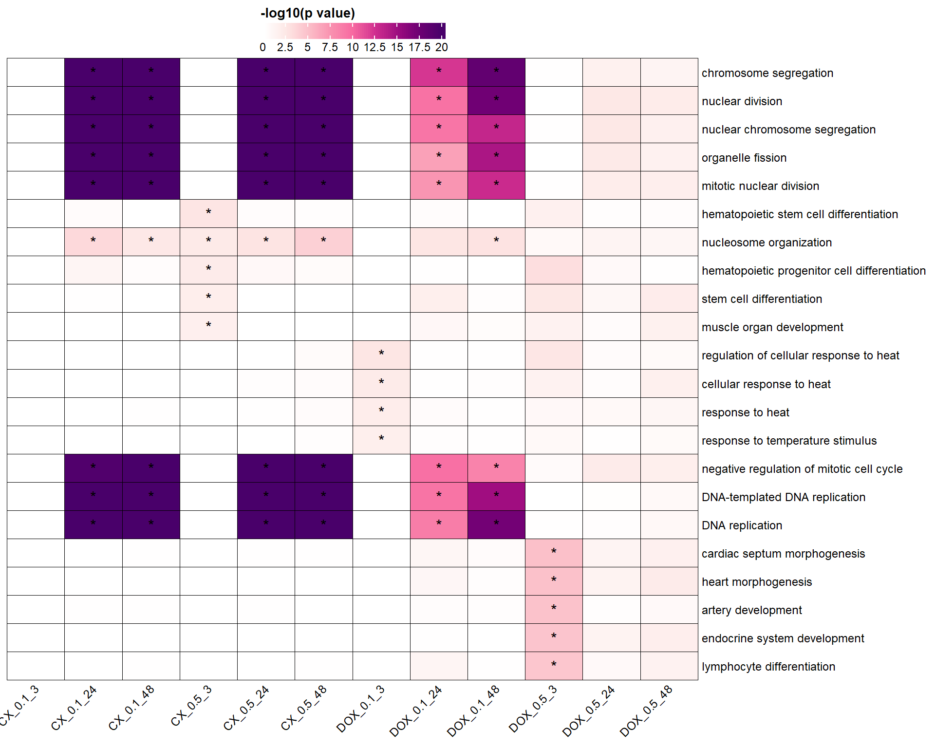
sessionInfo()R version 4.3.0 (2023-04-21 ucrt)
Platform: x86_64-w64-mingw32/x64 (64-bit)
Running under: Windows 11 x64 (build 26100)
Matrix products: default
locale:
[1] LC_COLLATE=English_United States.utf8
[2] LC_CTYPE=English_United States.utf8
[3] LC_MONETARY=English_United States.utf8
[4] LC_NUMERIC=C
[5] LC_TIME=English_United States.utf8
time zone: America/Chicago
tzcode source: internal
attached base packages:
[1] grid stats4 stats graphics grDevices utils datasets
[8] methods base
other attached packages:
[1] circlize_0.4.16
[2] ComplexHeatmap_2.18.0
[3] ReactomePA_1.46.0
[4] patchwork_1.3.0
[5] gprofiler2_0.2.3
[6] TxDb.Hsapiens.UCSC.hg38.knownGene_3.18.0
[7] RColorBrewer_1.1-3
[8] clusterProfiler_4.10.1
[9] pheatmap_1.0.12
[10] qvalue_2.34.0
[11] BiocParallel_1.36.0
[12] Homo.sapiens_1.3.1
[13] TxDb.Hsapiens.UCSC.hg19.knownGene_3.2.2
[14] org.Hs.eg.db_3.18.0
[15] GO.db_3.18.0
[16] OrganismDbi_1.44.0
[17] GenomicFeatures_1.54.4
[18] GenomicRanges_1.54.1
[19] GenomeInfoDb_1.38.8
[20] AnnotationDbi_1.64.1
[21] IRanges_2.36.0
[22] S4Vectors_0.40.2
[23] Biobase_2.62.0
[24] BiocGenerics_0.48.1
[25] edgeR_4.0.16
[26] limma_3.58.1
[27] cluster_2.1.8.1
[28] ggfortify_0.4.17
[29] lubridate_1.9.4
[30] forcats_1.0.0
[31] stringr_1.5.1
[32] dplyr_1.1.4
[33] purrr_1.0.4
[34] readr_2.1.5
[35] tidyr_1.3.1
[36] tibble_3.2.1
[37] ggplot2_3.5.2
[38] tidyverse_2.0.0
[39] workflowr_1.7.1
loaded via a namespace (and not attached):
[1] splines_4.3.0 later_1.3.2
[3] BiocIO_1.12.0 ggplotify_0.1.2
[5] bitops_1.0-9 filelock_1.0.3
[7] polyclip_1.10-7 graph_1.80.0
[9] XML_3.99-0.18 lifecycle_1.0.4
[11] doParallel_1.0.17 rprojroot_2.0.4
[13] processx_3.8.6 lattice_0.22-7
[15] MASS_7.3-60 magrittr_2.0.3
[17] plotly_4.10.4 sass_0.4.10
[19] rmarkdown_2.29 jquerylib_0.1.4
[21] yaml_2.3.10 httpuv_1.6.15
[23] cowplot_1.1.3 DBI_1.2.3
[25] abind_1.4-8 zlibbioc_1.48.2
[27] ggraph_2.2.1 RCurl_1.98-1.17
[29] yulab.utils_0.2.0 tweenr_2.0.3
[31] rappdirs_0.3.3 git2r_0.36.2
[33] GenomeInfoDbData_1.2.11 enrichplot_1.22.0
[35] ggrepel_0.9.6 tidytree_0.4.6
[37] reactome.db_1.86.2 codetools_0.2-20
[39] DelayedArray_0.28.0 DOSE_3.28.2
[41] xml2_1.3.8 ggforce_0.4.2
[43] shape_1.4.6.1 tidyselect_1.2.1
[45] aplot_0.2.5 farver_2.1.2
[47] viridis_0.6.5 matrixStats_1.5.0
[49] BiocFileCache_2.10.2 GenomicAlignments_1.38.2
[51] jsonlite_2.0.0 GetoptLong_1.0.5
[53] tidygraph_1.3.1 iterators_1.0.14
[55] foreach_1.5.2 tools_4.3.0
[57] progress_1.2.3 treeio_1.26.0
[59] Rcpp_1.0.12 glue_1.7.0
[61] gridExtra_2.3 SparseArray_1.2.4
[63] xfun_0.52 MatrixGenerics_1.14.0
[65] withr_3.0.2 BiocManager_1.30.25
[67] fastmap_1.2.0 callr_3.7.6
[69] digest_0.6.34 gridGraphics_0.5-1
[71] timechange_0.3.0 R6_2.6.1
[73] colorspace_2.1-0 Cairo_1.6-2
[75] biomaRt_2.58.2 RSQLite_2.3.9
[77] generics_0.1.3 data.table_1.17.0
[79] rtracklayer_1.62.0 htmlwidgets_1.6.4
[81] prettyunits_1.2.0 graphlayouts_1.2.2
[83] httr_1.4.7 S4Arrays_1.2.1
[85] scatterpie_0.2.4 graphite_1.48.0
[87] whisker_0.4.1 pkgconfig_2.0.3
[89] gtable_0.3.6 blob_1.2.4
[91] XVector_0.42.0 shadowtext_0.1.4
[93] htmltools_0.5.8.1 fgsea_1.28.0
[95] RBGL_1.78.0 clue_0.3-66
[97] scales_1.3.0 png_0.1-8
[99] ggfun_0.1.8 knitr_1.50
[101] rstudioapi_0.17.1 tzdb_0.5.0
[103] reshape2_1.4.4 rjson_0.2.23
[105] nlme_3.1-168 curl_6.2.2
[107] GlobalOptions_0.1.2 cachem_1.1.0
[109] parallel_4.3.0 HDO.db_0.99.1
[111] restfulr_0.0.15 pillar_1.10.2
[113] vctrs_0.6.5 promises_1.3.2
[115] dbplyr_2.5.0 evaluate_1.0.3
[117] magick_2.8.6 cli_3.6.1
[119] locfit_1.5-9.12 compiler_4.3.0
[121] Rsamtools_2.18.0 rlang_1.1.3
[123] crayon_1.5.3 labeling_0.4.3
[125] ps_1.8.1 getPass_0.2-4
[127] plyr_1.8.9 fs_1.6.3
[129] stringi_1.8.3 viridisLite_0.4.2
[131] munsell_0.5.1 Biostrings_2.70.3
[133] lazyeval_0.2.2 GOSemSim_2.28.1
[135] Matrix_1.6-1.1 hms_1.1.3
[137] bit64_4.6.0-1 KEGGREST_1.42.0
[139] statmod_1.5.0 SummarizedExperiment_1.32.0
[141] igraph_2.1.4 memoise_2.0.1
[143] bslib_0.9.0 ggtree_3.10.1
[145] fastmatch_1.1-6 bit_4.6.0
[147] gson_0.1.0 ape_5.8-1