Corrmotif Analysis
Last updated: 2025-02-27
Checks: 6 1
Knit directory: CX5461_Project/
This reproducible R Markdown analysis was created with workflowr (version 1.7.1). The Checks tab describes the reproducibility checks that were applied when the results were created. The Past versions tab lists the development history.
The R Markdown file has unstaged changes. To know which version of
the R Markdown file created these results, you’ll want to first commit
it to the Git repo. If you’re still working on the analysis, you can
ignore this warning. When you’re finished, you can run
wflow_publish to commit the R Markdown file and build the
HTML.
Great job! The global environment was empty. Objects defined in the global environment can affect the analysis in your R Markdown file in unknown ways. For reproduciblity it’s best to always run the code in an empty environment.
The command set.seed(20250129) was run prior to running
the code in the R Markdown file. Setting a seed ensures that any results
that rely on randomness, e.g. subsampling or permutations, are
reproducible.
Great job! Recording the operating system, R version, and package versions is critical for reproducibility.
Nice! There were no cached chunks for this analysis, so you can be confident that you successfully produced the results during this run.
Great job! Using relative paths to the files within your workflowr project makes it easier to run your code on other machines.
Great! You are using Git for version control. Tracking code development and connecting the code version to the results is critical for reproducibility.
The results in this page were generated with repository version 5429dbd. See the Past versions tab to see a history of the changes made to the R Markdown and HTML files.
Note that you need to be careful to ensure that all relevant files for
the analysis have been committed to Git prior to generating the results
(you can use wflow_publish or
wflow_git_commit). workflowr only checks the R Markdown
file, but you know if there are other scripts or data files that it
depends on. Below is the status of the Git repository when the results
were generated:
Ignored files:
    Ignored:    .RData
    Ignored:    .Rhistory
    Ignored:    .Rproj.user/
    Ignored:    analysis/figure/

Untracked files:
    Untracked:  data/Corrmotif/cormotif_all.RDS

Unstaged changes:
    Modified:   analysis/Corrmotif_all.Rmd
Note that any generated files, e.g. HTML, png, CSS, etc., are not included in this status report because it is ok for generated content to have uncommitted changes.
These are the previous versions of the repository in which changes were
made to the R Markdown (analysis/Corrmotif_all.Rmd) and
HTML (docs/Corrmotif_all.html) files. If you’ve configured
a remote Git repository (see ?wflow_git_remote), click on
the hyperlinks in the table below to view the files as they were in that
past version.
| File | Version | Author | Date | Message |
|---|---|---|---|---|
| Rmd | 4e8a4bc | sayanpaul01 | 2025-02-24 | Commit |
| html | 4e8a4bc | sayanpaul01 | 2025-02-24 | Commit |
| Rmd | 2862c42 | sayanpaul01 | 2025-02-24 | Commit |
| html | 2862c42 | sayanpaul01 | 2025-02-24 | Commit |
| Rmd | ebfddcd | sayanpaul01 | 2025-02-23 | Commit |
| html | ebfddcd | sayanpaul01 | 2025-02-23 | Commit |
| html | b557095 | sayanpaul01 | 2025-02-23 | Added CX_DOX shared late response (SVIP) boxplot |
| Rmd | 1cd333a | sayanpaul01 | 2025-02-23 | Added CX_DOX shared late response (SVIP) boxplot |
| html | e73d731 | sayanpaul01 | 2025-02-23 | Build site. |
| Rmd | c4ed3e0 | sayanpaul01 | 2025-02-23 | Updated Corrmotif analysis and index file |
| html | b56a62a | sayanpaul01 | 2025-02-21 | Build site. |
| Rmd | bf0c4a3 | sayanpaul01 | 2025-02-21 | Published updated Index and Corrmotif analysis with new |
📌 Fit Limma Model Functions
## Fit limma model using code as it is found in the original cormotif code. It has
## only been modified to add names to the matrix of t values, as well as the
## limma fits

limmafit.default <- function(exprs,groupid,compid) {
  limmafits  <- list()
  compnum    <- nrow(compid)
  genenum    <- nrow(exprs)
  limmat     <- matrix(0,genenum,compnum)
  limmas2    <- rep(0,compnum)
  limmadf    <- rep(0,compnum)
  limmav0    <- rep(0,compnum)
  limmag1num <- rep(0,compnum)
  limmag2num <- rep(0,compnum)

  rownames(limmat)  <- rownames(exprs)
  colnames(limmat)  <- rownames(compid)
  names(limmas2)    <- rownames(compid)
  names(limmadf)    <- rownames(compid)
  names(limmav0)    <- rownames(compid)
  names(limmag1num) <- rownames(compid)
  names(limmag2num) <- rownames(compid)

  for(i in 1:compnum) {
    selid1 <- which(groupid == compid[i,1])
    selid2 <- which(groupid == compid[i,2])
    eset   <- new("ExpressionSet", exprs=cbind(exprs[,selid1],exprs[,selid2]))
    g1num  <- length(selid1)
    g2num  <- length(selid2)
    designmat <- cbind(base=rep(1,(g1num+g2num)), delta=c(rep(0,g1num),rep(1,g2num)))
    fit <- lmFit(eset,designmat)
    fit <- eBayes(fit)
    limmat[,i] <- fit$t[,2]
    limmas2[i] <- fit$s2.prior
    limmadf[i] <- fit$df.prior
    limmav0[i] <- fit$var.prior[2]
    limmag1num[i] <- g1num
    limmag2num[i] <- g2num
    limmafits[[i]] <- fit

    # log odds
    # w<-sqrt(1+fit$var.prior[2]/(1/g1num+1/g2num))
    # log(0.99)+dt(fit$t[1,2],g1num+g2num-2+fit$df.prior,log=TRUE)-log(0.01)-dt(fit$t[1,2]/w, g1num+g2num-2+fit$df.prior, log=TRUE)+log(w)
  }
  names(limmafits) <- rownames(compid)
  limmacompnum<-nrow(compid)
  result<-list(t       = limmat,
               v0      = limmav0,
               df0     = limmadf,
               s20     = limmas2,
               g1num   = limmag1num,
               g2num   = limmag2num,
               compnum = limmacompnum,
               fits    = limmafits)
}

limmafit.counts <-
  function (exprs, groupid, compid, norm.factor.method = "TMM", voom.normalize.method = "none")
  {
    limmafits  <- list()
    compnum    <- nrow(compid)
    genenum    <- nrow(exprs)
    limmat     <- matrix(NA,genenum,compnum)
    limmas2    <- rep(0,compnum)
    limmadf    <- rep(0,compnum)
    limmav0    <- rep(0,compnum)
    limmag1num <- rep(0,compnum)
    limmag2num <- rep(0,compnum)

    rownames(limmat)  <- rownames(exprs)
    colnames(limmat)  <- rownames(compid)
    names(limmas2)    <- rownames(compid)
    names(limmadf)    <- rownames(compid)
    names(limmav0)    <- rownames(compid)
    names(limmag1num) <- rownames(compid)
    names(limmag2num) <- rownames(compid)

    for (i in 1:compnum) {
      message(paste("Running limma for comparision",i,"/",compnum))
      selid1 <- which(groupid == compid[i, 1])
      selid2 <- which(groupid == compid[i, 2])
      # make a new count data frame
      counts <- cbind(exprs[, selid1], exprs[, selid2])

      # remove NAs
      not.nas <- which(apply(counts, 1, function(x) !any(is.na(x))) == TRUE)

      # runn voom/limma
      d <- DGEList(counts[not.nas,])
      d <- calcNormFactors(d, method = norm.factor.method)
      g1num <- length(selid1)
      g2num <- length(selid2)
      designmat <- cbind(base = rep(1, (g1num + g2num)), delta = c(rep(0,
                                                                       g1num), rep(1, g2num)))

      y <- voom(d, designmat, normalize.method = voom.normalize.method)
      fit <- lmFit(y, designmat)
      fit <- eBayes(fit)

      limmafits[[i]] <- fit
      limmat[not.nas, i] <- fit$t[, 2]
      limmas2[i] <- fit$s2.prior
      limmadf[i] <- fit$df.prior
      limmav0[i] <- fit$var.prior[2]
      limmag1num[i] <- g1num
      limmag2num[i] <- g2num
    }
    limmacompnum <- nrow(compid)
    names(limmafits) <- rownames(compid)
    result <- list(t       = limmat,
                   v0      = limmav0,
                   df0     = limmadf,
                   s20     = limmas2,
                   g1num   = limmag1num,
                   g2num   = limmag2num,
                   compnum = limmacompnum,
                   fits    = limmafits)
  }

limmafit.list <-
  function (fitlist, cmp.idx=2)
  {
    compnum    <- length(fitlist)

    genes <- c()
    for (i in 1:compnum) genes <- unique(c(genes, rownames(fitlist[[i]])))

    genenum    <- length(genes)
    limmat     <- matrix(NA,genenum,compnum)
    limmas2    <- rep(0,compnum)
    limmadf    <- rep(0,compnum)
    limmav0    <- rep(0,compnum)
    limmag1num <- rep(0,compnum)
    limmag2num <- rep(0,compnum)

    rownames(limmat)  <- genes
    colnames(limmat)  <- names(fitlist)
    names(limmas2)    <- names(fitlist)
    names(limmadf)    <- names(fitlist)
    names(limmav0)    <- names(fitlist)
    names(limmag1num) <- names(fitlist)
    names(limmag2num) <- names(fitlist)

    for (i in 1:compnum) {
      this.t <- fitlist[[i]]$t[,cmp.idx]
      limmat[names(this.t),i] <- this.t

      limmas2[i]    <- fitlist[[i]]$s2.prior
      limmadf[i]    <- fitlist[[i]]$df.prior
      limmav0[i]    <- fitlist[[i]]$var.prior[cmp.idx]
      limmag1num[i] <- sum(fitlist[[i]]$design[,cmp.idx]==0)
      limmag2num[i] <- sum(fitlist[[i]]$design[,cmp.idx]==1)
    }

    limmacompnum <- compnum
    result <- list(t       = limmat,
                   v0      = limmav0,
                   df0     = limmadf,
                   s20     = limmas2,
                   g1num   = limmag1num,
                   g2num   = limmag2num,
                   compnum = limmacompnum,
                   fits    = limmafits)

  }

## Rank genes based on statistics
generank<-function(x) {
  xcol<-ncol(x)
  xrow<-nrow(x)
  result<-matrix(0,xrow,xcol)
  z<-(1:1:xrow)
  for(i in 1:xcol) {
    y<-sort(x[,i],decreasing=TRUE,na.last=TRUE)
    result[,i]<-match(x[,i],y)
    result[,i]<-order(result[,i])
  }
  result
}

## Log-likelihood for moderated t under H0
modt.f0.loglike<-function(x,df) {
  a<-dt(x, df, log=TRUE)
  result<-as.vector(a)
  flag<-which(is.na(result)==TRUE)
  result[flag]<-0
  result
}

## Log-likelihood for moderated t under H1
## param=c(df,g1num,g2num,v0)
modt.f1.loglike<-function(x,param) {
  df<-param[1]
  g1num<-param[2]
  g2num<-param[3]
  v0<-param[4]
  w<-sqrt(1+v0/(1/g1num+1/g2num))
  dt(x/w, df, log=TRUE)-log(w)
  a<-dt(x/w, df, log=TRUE)-log(w)
  result<-as.vector(a)
  flag<-which(is.na(result)==TRUE)
  result[flag]<-0
  result
}

## Correlation Motif Fit
cmfit.X<-function(x, type, K=1, tol=1e-3, max.iter=100) {
  ## initialize
  xrow <- nrow(x)
  xcol <- ncol(x)
  loglike0 <- list()
  loglike1 <- list()
  p <- rep(1, K)/K
  q <- matrix(runif(K * xcol), K, xcol)
  q[1, ] <- rep(0.01, xcol)
  for (i in 1:xcol) {
    f0 <- type[[i]][[1]]
    f0param <- type[[i]][[2]]
    f1 <- type[[i]][[3]]
    f1param <- type[[i]][[4]]
    loglike0[[i]] <- f0(x[, i], f0param)
    loglike1[[i]] <- f1(x[, i], f1param)
  }
  condlike <- list()
  for (i in 1:xcol) {
    condlike[[i]] <- matrix(0, xrow, K)
  }
  loglike.old <- -1e+10
  for (i.iter in 1:max.iter) {
    if ((i.iter%%50) == 0) {
      print(paste("We have run the first ", i.iter, " iterations for K=",
                  K, sep = ""))
    }
    err <- tol + 1
    clustlike <- matrix(0, xrow, K)
    #templike <- matrix(0, xrow, 2)
    templike1 <- rep(0, xrow)
    templike2 <- rep(0, xrow)
    for (j in 1:K) {
      for (i in 1:xcol) {
        templike1 <- log(q[j, i]) + loglike1[[i]]
        templike2 <- log(1 - q[j, i]) + loglike0[[i]]
        tempmax <- Rfast::Pmax(templike1, templike2)

        templike1 <- exp(templike1 - tempmax)
        templike2 <- exp(templike2 - tempmax)

        tempsum <- templike1 + templike2
        clustlike[, j] <- clustlike[, j] + tempmax +
          log(tempsum)
        condlike[[i]][, j] <- templike1/tempsum
      }
      clustlike[, j] <- clustlike[, j] + log(p[j])
    }
    #tempmax <- apply(clustlike, 1, max)
    tempmax <- Rfast::rowMaxs(clustlike, value=TRUE)
    for (j in 1:K) {
      clustlike[, j] <- exp(clustlike[, j] - tempmax)
    }
    #tempsum <- apply(clustlike, 1, sum)
    tempsum <- Rfast::rowsums(clustlike)
    for (j in 1:K) {
      clustlike[, j] <- clustlike[, j]/tempsum
    }
    #p.new <- (apply(clustlike, 2, sum) + 1)/(xrow + K)
    p.new <- (Rfast::colsums(clustlike) + 1)/(xrow + K)
    q.new <- matrix(0, K, xcol)
    for (j in 1:K) {
      clustpsum <- sum(clustlike[, j])
      for (i in 1:xcol) {
        q.new[j, i] <- (sum(clustlike[, j] * condlike[[i]][,
                                                           j]) + 1)/(clustpsum + 2)
      }
    }
    err.p <- max(abs(p.new - p)/p)
    err.q <- max(abs(q.new - q)/q)
    err <- max(err.p, err.q)
    loglike.new <- (sum(tempmax + log(tempsum)) + sum(log(p.new)) +
                      sum(log(q.new) + log(1 - q.new)))/xrow
    p <- p.new
    q <- q.new
    loglike.old <- loglike.new
    if (err < tol) {
      break
    }
  }
  clustlike <- matrix(0, xrow, K)
  for (j in 1:K) {
    for (i in 1:xcol) {
      templike1 <- log(q[j, i]) + loglike1[[i]]
      templike2 <- log(1 - q[j, i]) + loglike0[[i]]
      tempmax <- Rfast::Pmax(templike1, templike2)

      templike1 <- exp(templike1 - tempmax)
      templike2 <- exp(templike2 - tempmax)

      tempsum <- templike1 + templike2
      clustlike[, j] <- clustlike[, j] + tempmax + log(tempsum)
      condlike[[i]][, j] <- templike1/tempsum
    }
    clustlike[, j] <- clustlike[, j] + log(p[j])
  }
  #tempmax <- apply(clustlike, 1, max)
  tempmax <- Rfast::rowMaxs(clustlike, value=TRUE)
  for (j in 1:K) {
    clustlike[, j] <- exp(clustlike[, j] - tempmax)
  }
  #tempsum <- apply(clustlike, 1, sum)
  tempsum <- Rfast::rowsums(clustlike)
  for (j in 1:K) {
    clustlike[, j] <- clustlike[, j]/tempsum
  }
  p.post <- matrix(0, xrow, xcol)
  for (j in 1:K) {
    for (i in 1:xcol) {
      p.post[, i] <- p.post[, i] + clustlike[, j] * condlike[[i]][,
                                                                  j]
    }
  }
  loglike.old <- loglike.old - (sum(log(p)) + sum(log(q) +
                                                    log(1 - q)))/xrow
  loglike.old <- loglike.old * xrow
  result <- list(p.post = p.post, motif.prior = p, motif.q = q,
                 loglike = loglike.old, clustlike=clustlike, condlike=condlike)
}

## Fit using (0,0,...,0) and (1,1,...,1)
cmfitall<-function(x, type, tol=1e-3, max.iter=100) {
  ## initialize
  xrow<-nrow(x)
  xcol<-ncol(x)
  loglike0<-list()
  loglike1<-list()
  p<-0.01

  ## compute loglikelihood
  L0<-matrix(0,xrow,1)
  L1<-matrix(0,xrow,1)
  for(i in 1:xcol) {
    f0<-type[[i]][[1]]
    f0param<-type[[i]][[2]]
    f1<-type[[i]][[3]]
    f1param<-type[[i]][[4]]
    loglike0[[i]]<-f0(x[,i],f0param)
    loglike1[[i]]<-f1(x[,i],f1param)
    L0<-L0+loglike0[[i]]
    L1<-L1+loglike1[[i]]
  }


  ## EM algorithm to get MLE of p and q
  loglike.old <- -1e10
  for(i.iter in 1:max.iter) {
    if((i.iter%%50) == 0) {
      print(paste("We have run the first ", i.iter, " iterations",sep=""))
    }
    err<-tol+1

    ## compute posterior cluster membership
    clustlike<-matrix(0,xrow,2)
    clustlike[,1]<-log(1-p)+L0
    clustlike[,2]<-log(p)+L1

    tempmax<-apply(clustlike,1,max)
    for(j in 1:2) {
      clustlike[,j]<-exp(clustlike[,j]-tempmax)
    }
    tempsum<-apply(clustlike,1,sum)

    ## update motif occurrence rate
    for(j in 1:2) {
      clustlike[,j]<-clustlike[,j]/tempsum
    }

    p.new<-(sum(clustlike[,2])+1)/(xrow+2)

    ## evaluate convergence
    err<-abs(p.new-p)/p

    ## evaluate whether the log.likelihood increases
    loglike.new<-(sum(tempmax+log(tempsum))+log(p.new)+log(1-p.new))/xrow

    loglike.old<-loglike.new
    p<-p.new

    if(err<tol) {
      break;
    }
  }

  ## compute posterior p
  clustlike<-matrix(0,xrow,2)
  clustlike[,1]<-log(1-p)+L0
  clustlike[,2]<-log(p)+L1

  tempmax<-apply(clustlike,1,max)
  for(j in 1:2) {
    clustlike[,j]<-exp(clustlike[,j]-tempmax)
  }
  tempsum<-apply(clustlike,1,sum)

  for(j in 1:2) {
    clustlike[,j]<-clustlike[,j]/tempsum
  }

  p.post<-matrix(0,xrow,xcol)
  for(i in 1:xcol) {
    p.post[,i]<-clustlike[,2]
  }

  ## return

  #calculate back loglikelihood
  loglike.old<-loglike.old-(log(p)+log(1-p))/xrow
  loglike.old<-loglike.old*xrow
  result<-list(p.post=p.post, motif.prior=p, loglike=loglike.old)
}

## Fit each dataset separately
cmfitsep<-function(x, type, tol=1e-3, max.iter=100) {
  ## initialize
  xrow<-nrow(x)
  xcol<-ncol(x)
  loglike0<-list()
  loglike1<-list()
  p<-0.01*rep(1,xcol)
  loglike.final<-rep(0,xcol)

  ## compute loglikelihood
  for(i in 1:xcol) {
    f0<-type[[i]][[1]]
    f0param<-type[[i]][[2]]
    f1<-type[[i]][[3]]
    f1param<-type[[i]][[4]]
    loglike0[[i]]<-f0(x[,i],f0param)
    loglike1[[i]]<-f1(x[,i],f1param)
  }

  p.post<-matrix(0,xrow,xcol)

  ## EM algorithm to get MLE of p
  for(coli in 1:xcol) {
    loglike.old <- -1e10
    for(i.iter in 1:max.iter) {
      if((i.iter%%50) == 0) {
        print(paste("We have run the first ", i.iter, " iterations",sep=""))
      }
      err<-tol+1

      ## compute posterior cluster membership
      clustlike<-matrix(0,xrow,2)
      clustlike[,1]<-log(1-p[coli])+loglike0[[coli]]
      clustlike[,2]<-log(p[coli])+loglike1[[coli]]

      tempmax<-apply(clustlike,1,max)
      for(j in 1:2) {
        clustlike[,j]<-exp(clustlike[,j]-tempmax)
      }
      tempsum<-apply(clustlike,1,sum)

      ## evaluate whether the log.likelihood increases
      loglike.new<-sum(tempmax+log(tempsum))/xrow

      ## update motif occurrence rate
      for(j in 1:2) {
        clustlike[,j]<-clustlike[,j]/tempsum
      }

      p.new<-(sum(clustlike[,2]))/(xrow)

      ## evaluate convergence
      err<-abs(p.new-p[coli])/p[coli]
      loglike.old<-loglike.new
      p[coli]<-p.new

      if(err<tol) {
        break;
      }
    }

    ## compute posterior p
    clustlike<-matrix(0,xrow,2)
    clustlike[,1]<-log(1-p[coli])+loglike0[[coli]]
    clustlike[,2]<-log(p[coli])+loglike1[[coli]]

    tempmax<-apply(clustlike,1,max)
    for(j in 1:2) {
      clustlike[,j]<-exp(clustlike[,j]-tempmax)
    }
    tempsum<-apply(clustlike,1,sum)

    for(j in 1:2) {
      clustlike[,j]<-clustlike[,j]/tempsum
    }

    p.post[,coli]<-clustlike[,2]
    loglike.final[coli]<-loglike.old
  }


  ## return
  loglike.final<-loglike.final*xrow
  result<-list(p.post=p.post, motif.prior=p, loglike=loglike.final)
}

## Fit the full model
cmfitfull<-function(x, type, tol=1e-3, max.iter=100) {
  ## initialize
  xrow<-nrow(x)
  xcol<-ncol(x)
  loglike0<-list()
  loglike1<-list()
  K<-2^xcol
  p<-rep(1,K)/K
  pattern<-rep(0,xcol)
  patid<-matrix(0,K,xcol)

  ## compute loglikelihood
  for(i in 1:xcol) {
    f0<-type[[i]][[1]]
    f0param<-type[[i]][[2]]
    f1<-type[[i]][[3]]
    f1param<-type[[i]][[4]]
    loglike0[[i]]<-f0(x[,i],f0param)
    loglike1[[i]]<-f1(x[,i],f1param)
  }
  L<-matrix(0,xrow,K)
  for(i in 1:K)
  {
    patid[i,]<-pattern
    for(j in 1:xcol) {
      if(pattern[j] < 0.5) {
        L[,i]<-L[,i]+loglike0[[j]]
      } else {
        L[,i]<-L[,i]+loglike1[[j]]
      }
    }

    if(i < K) {
      pattern[xcol]<-pattern[xcol]+1
      j<-xcol
      while(pattern[j] > 1) {
        pattern[j]<-0
        j<-j-1
        pattern[j]<-pattern[j]+1
      }
    }
  }

  ## EM algorithm to get MLE of p and q
  loglike.old <- -1e10
  for(i.iter in 1:max.iter) {
    if((i.iter%%50) == 0) {
      print(paste("We have run the first ", i.iter, " iterations",sep=""))
    }
    err<-tol+1

    ## compute posterior cluster membership
    clustlike<-matrix(0,xrow,K)
    for(j in 1:K) {
      clustlike[,j]<-log(p[j])+L[,j]
    }

    tempmax<-apply(clustlike,1,max)
    for(j in 1:K) {
      clustlike[,j]<-exp(clustlike[,j]-tempmax)
    }
    tempsum<-apply(clustlike,1,sum)

    ## update motif occurrence rate
    for(j in 1:K) {
      clustlike[,j]<-clustlike[,j]/tempsum
    }

    p.new<-(apply(clustlike,2,sum)+1)/(xrow+K)

    ## evaluate convergence
    err<-max(abs(p.new-p)/p)

    ## evaluate whether the log.likelihood increases
    loglike.new<-(sum(tempmax+log(tempsum))+sum(log(p.new)))/xrow

    loglike.old<-loglike.new
    p<-p.new

    if(err<tol) {
      break;
    }
  }

  ## compute posterior p
  clustlike<-matrix(0,xrow,K)
  for(j in 1:K) {
    clustlike[,j]<-log(p[j])+L[,j]
  }

  tempmax<-apply(clustlike,1,max)
  for(j in 1:K) {
    clustlike[,j]<-exp(clustlike[,j]-tempmax)
  }
  tempsum<-apply(clustlike,1,sum)

  for(j in 1:K) {
    clustlike[,j]<-clustlike[,j]/tempsum
  }

  p.post<-matrix(0,xrow,xcol)
  for(j in 1:K) {
    for(i in 1:xcol) {
      if(patid[j,i] > 0.5) {
        p.post[,i]<-p.post[,i]+clustlike[,j]
      }
    }
  }

  ## return
  #calculate back loglikelihood
  loglike.old<-loglike.old-sum(log(p))/xrow
  loglike.old<-loglike.old*xrow
  result<-list(p.post=p.post, motif.prior=p, loglike=loglike.old)
}

generatetype<-function(limfitted)
{
  jtype<-list()
  df<-limfitted$g1num+limfitted$g2num-2+limfitted$df0
  for(j in 1:limfitted$compnum)
  {
    jtype[[j]]<-list(f0=modt.f0.loglike, f0.param=df[j], f1=modt.f1.loglike, f1.param=c(df[j],limfitted$g1num[j],limfitted$g2num[j],limfitted$v0[j]))
  }
  jtype
}

cormotiffit <- function(exprs, groupid=NULL, compid=NULL, K=1, tol=1e-3,
                        max.iter=100, BIC=TRUE, norm.factor.method="TMM",
                        voom.normalize.method = "none", runtype=c("logCPM","counts","limmafits"), each=3)
{
  # first I want to do some typechecking. Input can be either a normalized
  # matrix, a count matrix, or a list of limma fits. Dispatch the correct
  # limmafit accordingly.
  # todo: add some typechecking here
  limfitted <- list()
  if (runtype=="counts") {
    limfitted <- limmafit.counts(exprs,groupid,compid, norm.factor.method, voom.normalize.method)
  } else if (runtype=="logCPM") {
    limfitted <- limmafit.default(exprs,groupid,compid)
  } else if (runtype=="limmafits") {
    limfitted <- limmafit.list(exprs)
  } else {
    stop("runtype must be one of 'logCPM', 'counts', or 'limmafits'")
  }


  jtype<-generatetype(limfitted)
  fitresult<-list()
  ks <- rep(K, each = each)
  fitresult <- bplapply(1:length(ks), function(i, x, type, ks, tol, max.iter) {
    cmfit.X(x, type, K = ks[i], tol = tol, max.iter = max.iter)
  }, x=limfitted$t, type=jtype, ks=ks, tol=tol, max.iter=max.iter)

  best.fitresults <- list()
  for (i in 1:length(K)) {
    w.k <- which(ks==K[i])
    this.bic <- c()
    for (j in w.k) this.bic[j] <- -2 * fitresult[[j]]$loglike + (K[i] - 1 + K[i] * limfitted$compnum) * log(dim(limfitted$t)[1])
    w.min <- which(this.bic == min(this.bic, na.rm = TRUE))[1]
    best.fitresults[[i]] <- fitresult[[w.min]]
  }
  fitresult <- best.fitresults

  bic <- rep(0, length(K))
  aic <- rep(0, length(K))
  loglike <- rep(0, length(K))
  for (i in 1:length(K)) loglike[i] <- fitresult[[i]]$loglike
  for (i in 1:length(K)) bic[i] <- -2 * fitresult[[i]]$loglike + (K[i] - 1 + K[i] * limfitted$compnum) * log(dim(limfitted$t)[1])
  for (i in 1:length(K)) aic[i] <- -2 * fitresult[[i]]$loglike + 2 * (K[i] - 1 + K[i] * limfitted$compnum)
  if(BIC==TRUE) {
    bestflag=which(bic==min(bic))
  }
  else {
    bestflag=which(aic==min(aic))
  }
  result<-list(bestmotif=fitresult[[bestflag]],bic=cbind(K,bic),
               aic=cbind(K,aic),loglike=cbind(K,loglike), allmotifs=fitresult)

}

cormotiffitall<-function(exprs,groupid,compid, tol=1e-3, max.iter=100)
{
  limfitted<-limmafit(exprs,groupid,compid)
  jtype<-generatetype(limfitted)
  fitresult<-cmfitall(limfitted$t,type=jtype,tol=1e-3,max.iter=max.iter)
}

cormotiffitsep<-function(exprs,groupid,compid, tol=1e-3, max.iter=100)
{
  limfitted<-limmafit(exprs,groupid,compid)
  jtype<-generatetype(limfitted)
  fitresult<-cmfitsep(limfitted$t,type=jtype,tol=1e-3,max.iter=max.iter)
}

cormotiffitfull<-function(exprs,groupid,compid, tol=1e-3, max.iter=100)
{
  limfitted<-limmafit(exprs,groupid,compid)
  jtype<-generatetype(limfitted)
  fitresult<-cmfitfull(limfitted$t,type=jtype,tol=1e-3,max.iter=max.iter)
}

plotIC<-function(fitted_cormotif)
{
  oldpar<-par(mfrow=c(1,2))
  plot(fitted_cormotif$bic[,1], fitted_cormotif$bic[,2], type="b",xlab="Motif Number", ylab="BIC", main="BIC")
  plot(fitted_cormotif$aic[,1], fitted_cormotif$aic[,2], type="b",xlab="Motif Number", ylab="AIC", main="AIC")
}

plotMotif<-function(fitted_cormotif,title="")
{
  layout(matrix(1:2,ncol=2))
  u<-1:dim(fitted_cormotif$bestmotif$motif.q)[2]
  v<-1:dim(fitted_cormotif$bestmotif$motif.q)[1]
  image(u,v,t(fitted_cormotif$bestmotif$motif.q),
        col=gray(seq(from=1,to=0,by=-0.1)),xlab="Study",yaxt = "n",
        ylab="Corr. Motifs",main=paste(title,"pattern",sep=" "))
  axis(2,at=1:length(v))
  for(i in 1:(length(u)+1))
  {
    abline(v=(i-0.5))
  }
  for(i in 1:(length(v)+1))
  {
    abline(h=(i-0.5))
  }
  Ng=10000
  if(is.null(fitted_cormotif$bestmotif$p.post)!=TRUE)
    Ng=nrow(fitted_cormotif$bestmotif$p.post)
  genecount=floor(fitted_cormotif$bestmotif$motif.p*Ng)
  NK=nrow(fitted_cormotif$bestmotif$motif.q)
  plot(0,0.7,pch=".",xlim=c(0,1.2),ylim=c(0.75,NK+0.25),
       frame.plot=FALSE,axes=FALSE,xlab="No. of genes",ylab="", main=paste(title,"frequency",sep=" "))
  segments(0,0.7,fitted_cormotif$bestmotif$motif.p[1],0.7)
  rect(0,1:NK-0.3,fitted_cormotif$bestmotif$motif.p,1:NK+0.3,
       col="dark grey")
  mtext(1:NK,at=1:NK,side=2,cex=0.8)
  text(fitted_cormotif$bestmotif$motif.p+0.15,1:NK,
       labels=floor(fitted_cormotif$bestmotif$motif.p*Ng))
}
📌 Load Required Libraries
library(tidyverse)
library(ggplot2)
library(tidyr)
library(dplyr)
library(reshape2)
library(clusterProfiler)
library(AnnotationDbi)
library(org.Hs.eg.db)
library(RColorBrewer)
library(gprofiler2)
library(pheatmap)
library(ggpubr)
library(corrplot)
library(Cormotif)
library(Rfast)
library(BiocParallel)
📌 Load Corrmotif Data
# Read the Corrmotif Results
Corrmotif <- read.csv("data/Corrmotif/CX5461.csv")
Corrmotif_df <- data.frame(Corrmotif)

rownames(Corrmotif_df) <- Corrmotif_df$Gene
exprs.corrmotif <- as.matrix(Corrmotif_df[,2:109])

# Read group and comparison IDs
groupid_df <- read.csv("data/Corrmotif/groupid.csv")
compid_df <- read.csv("data/Corrmotif/Compid.csv")
📌 Fit Corrmotif Model (K=1:8)
set.seed(11111)
# Fit Corrmotif Model (K = 1 to 8)
set.seed(11111)
motif.fitted <- cormotiffit(
  exprs = exprs.corrmotif,
  groupid = groupid_df,
  compid = compid_df,
  K = 1:8,
  max.iter = 1000,
  BIC = TRUE,
  runtype = "logCPM"
)

gene_prob_all <- motif.fitted$bestmotif$p.post
rownames(gene_prob_all) <- rownames(Corrmotif_df)
motif_prob <- motif.fitted$bestmotif$clustlike
rownames(motif_prob) <- rownames(gene_prob_all)
write.csv(motif_prob,"data/cormotif_probability_genelist_all.csv")
📌 Plot motif
cormotif_all <- readRDS("data/Corrmotif/cormotif_all.RDS")
cormotif_all$bic
K bic
[1,] 1 643837.2
[2,] 2 632515.2
[3,] 3 626572.5
[4,] 4 624577.2
[5,] 5 624656.6
[6,] 6 624667.6
[7,] 7 624660.0
[8,] 8 624786.5plotIC(cormotif_all)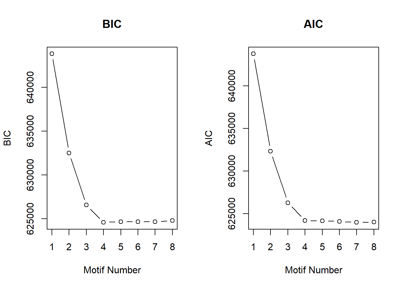
plotMotif(cormotif_all)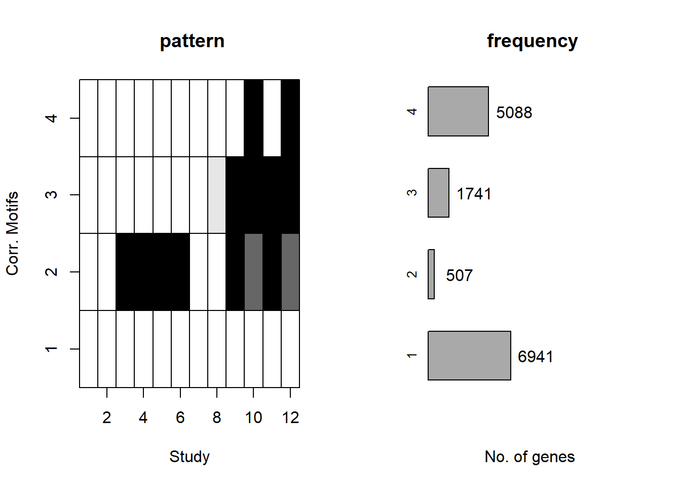
📌 Extract Gene Probabilities
# Extract posterior probabilities for genes
gene_prob_all <- cormotif_all$bestmotif$p.post
rownames(gene_prob_all) <- rownames(Corrmotif_df)

# Define gene probability groups
prob_all_1  <- rownames(gene_prob_all[(gene_prob_all[,1] <0.5 & gene_prob_all[,2] <0.5 & gene_prob_all[,3] <0.5 & gene_prob_all[,4] <0.5 & gene_prob_all[,5] < 0.5 & gene_prob_all[,6]<0.5 & gene_prob_all[,7]<0.5 & gene_prob_all[,8]<0.5 & gene_prob_all[,9]<0.5 & gene_prob_all[,10]<0.5 & gene_prob_all[,11]<0.5 & gene_prob_all[,12]<0.5),])

length(prob_all_1)

prob_all_2  <- rownames(gene_prob_all[(gene_prob_all[,1] <0.5 & gene_prob_all[,2] <0.5 & gene_prob_all[,3] >0.5 & gene_prob_all[,4] >0.5 & gene_prob_all[,5] > 0.5 & gene_prob_all[,6]>0.5 & gene_prob_all[,7]<0.5 & gene_prob_all[,8]<0.5 & gene_prob_all[,9]>0.5 & gene_prob_all[,10]>0.1 & gene_prob_all[,11]>0.5 & gene_prob_all[,12]>0.1),])

length(prob_all_2)

prob_all_3  <- rownames(gene_prob_all[(gene_prob_all[,1] <0.5 & gene_prob_all[,2] <0.5 & gene_prob_all[,3] <0.5 & gene_prob_all[,4] <0.5 & gene_prob_all[,5] < 0.5 & gene_prob_all[,6]<0.5 & gene_prob_all[,7]<0.5 & gene_prob_all[,8]>=0.02 & gene_prob_all[,9]>0.5 & gene_prob_all[,10]>0.5 & gene_prob_all[,11]>0.5 & gene_prob_all[,12]>0.5),])

length(prob_all_3)

prob_all_4  <- rownames(gene_prob_all[(gene_prob_all[,1] <0.5 & gene_prob_all[,2] <0.5 & gene_prob_all[,3] <0.5 & gene_prob_all[,4] <0.5 & gene_prob_all[,5] < 0.5 & gene_prob_all[,6]<0.5 & gene_prob_all[,7]<0.5 & gene_prob_all[,8]<0.5 & gene_prob_all[,9]<0.5 & gene_prob_all[,10]>0.5 & gene_prob_all[,11]<0.5 & gene_prob_all[,12]>0.5),])

length(prob_all_4)
📌 Distribution of Gene Clusters Identified by Corrmotif
# Load necessary library
library(ggplot2)

# Data
data <- data.frame(
  Category = c("Non response", "CX_DOX shared late response",
               "Dox specific response", "Late high dose DOX specific response"),
  Value = c(7031, 414, 1531, 4874)
)

# Define custom colors
custom_colors <- c("Non response" = "#FF9999",
                   "CX_DOX shared late response" = "#66B2FF",
                   "Dox specific response" = "#99FF99",
                   "Late high dose DOX specific response" = "#FFD700")

# Create pie chart
ggplot(data, aes(x = "", y = Value, fill = Category)) +
  geom_bar(width = 1, stat = "identity") +
  coord_polar("y", start = 0) +
  geom_text(aes(label = Value),
            position = position_stack(vjust = 0.5),
            size = 4, color = "black") +
  labs(title = "Distribution of Gene Clusters Identified by Corrmotif", x = NULL, y = NULL) +
  theme_void() +
  scale_fill_manual(values = custom_colors)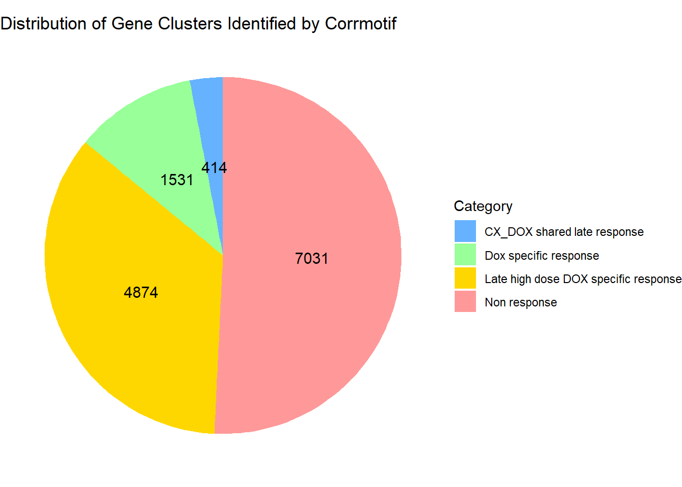
| Version | Author | Date |
|---|---|---|
| b56a62a | sayanpaul01 | 2025-02-21 |
📌 Corr-motif Boxplots
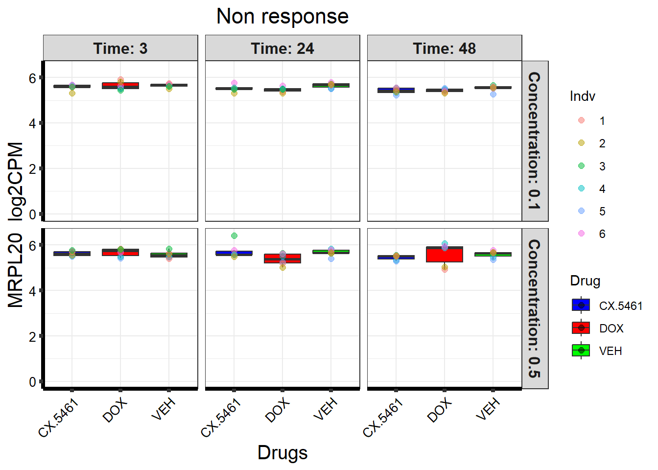
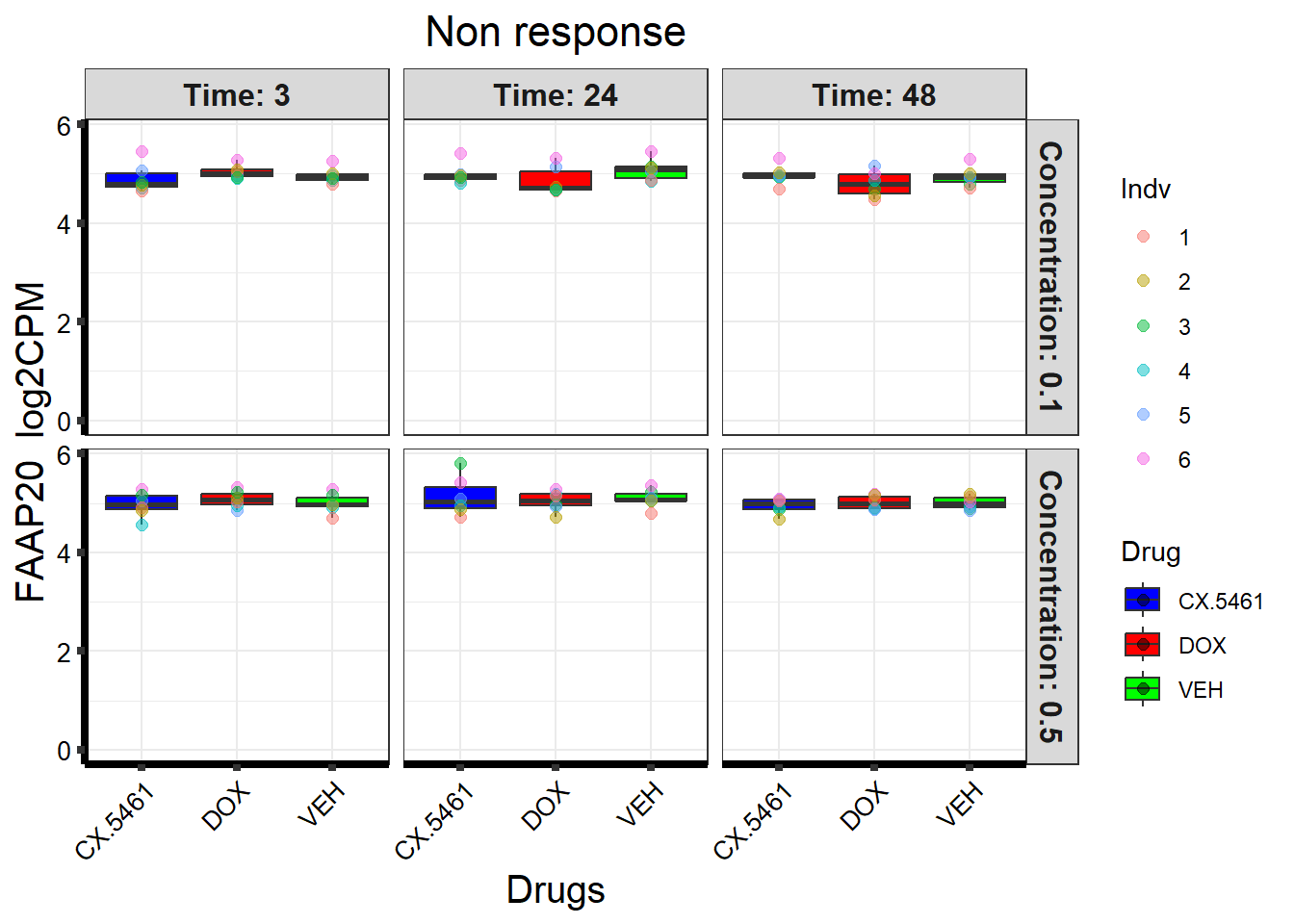
📌 Non response (MRPL20)
# Load the dataset from the data folder
# Load the dataset from the data folder
boxplot1 <- read.csv("data/boxplot1.csv", check.names = FALSE)

boxplot1 <- as.data.frame(boxplot1)

# Print first few column names to check structure
print(colnames(boxplot1))
[1] "" "ENTREZID" "SYMBOL"
[4] "GENENAME" "17.3_CX.5461_0.1_3" "17.3_DOX_0.5_24"
[7] "87.1_DOX_0.5_24" "87.1_VEH_0.1_24" "87.1_VEH_0.5_24"
[10] "87.1_CX.5461_0.1_48" "87.1_CX.5461_0.5_48" "87.1_DOX_0.1_48"
[13] "87.1_DOX_0.5_48" "87.1_VEH_0.1_48" "87.1_VEH_0.5_48"
[16] "17.3_VEH_0.1_24" "17.3_VEH_0.5_24" "17.3_CX.5461_0.1_48"
[19] "17.3_CX.5461_0.5_48" "17.3_DOX_0.1_48" "17.3_DOX_0.5_48"
[22] "17.3_VEH_0.1_48" "17.3_VEH_0.5_48" "84.1_CX.5461_0.1_3"
[25] "17.3_CX.5461_0.5_3" "84.1_CX.5461_0.5_3" "84.1_DOX_0.1_3"
[28] "84.1_DOX_0.5_3" "84.1_VEH_0.1_3" "84.1_VEH_0.5_3"
[31] "84.1_CX.5461_0.1_24" "84.1_CX.5461_0.5_24" "84.1_DOX_0.1_24"
[34] "84.1_DOX_0.5_24" "84.1_VEH_0.1_24" "17.3_DOX_0.1_3"
[37] "84.1_VEH_0.5_24" "84.1_CX.5461_0.1_48" "84.1_CX.5461_0.5_48"
[40] "84.1_DOX_0.1_48" "84.1_DOX_0.5_48" "84.1_VEH_0.1_48"
[43] "84.1_VEH_0.5_48" "90.1_CX.5461_0.1_3" "90.1_CX.5461_0.5_3"
[46] "90.1_DOX_0.1_3" "17.3_DOX_0.5_3" "90.1_DOX_0.5_3"
[49] "90.1_VEH_0.1_3" "90.1_VEH_0.5_3" "90.1_CX.5461_0.1_24"
[52] "90.1_CX.5461_0.5_24" "90.1_DOX_0.1_24" "90.1_DOX_0.5_24"
[55] "90.1_VEH_0.1_24" "90.1_VEH_0.5_24" "90.1_CX.5461_0.1_48"
[58] "17.3_VEH_0.1_3" "90.1_CX.5461_0.5_48" "90.1_DOX_0.1_48"
[61] "90.1_DOX_0.5_48" "90.1_VEH_0.1_48" "90.1_VEH_0.5_48"
[64] "75.1_CX.5461_0.1_3" "75.1_CX.5461_0.5_3" "75.1_DOX_0.1_3"
[67] "75.1_DOX_0.5_3" "75.1_VEH_0.1_3" "17.3_VEH_0.5_3"
[70] "75.1_VEH_0.5_3" "75.1_CX.5461_0.1_24" "75.1_CX.5461_0.5_24"
[73] "75.1_DOX_0.1_24" "75.1_DOX_0.5_24" "75.1_VEH_0.1_24"
[76] "75.1_VEH_0.5_24" "75.1_CX.5461_0.1_48" "75.1_CX.5461_0.5_48"
[79] "75.1_DOX_0.1_48" "17.3_CX.5461_0.1_24" "75.1_DOX_0.5_48"
[82] "75.1_VEH_0.1_48" "75.1_VEH_0.5_48" "78.1_CX.5461_0.1_3"
[85] "78.1_CX.5461_0.5_3" "78.1_DOX_0.1_3" "78.1_DOX_0.5_3"
[88] "78.1_VEH_0.1_3" "78.1_VEH_0.5_3" "78.1_CX.5461_0.1_24"
[91] "17.3_CX.5461_0.5_24" "78.1_CX.5461_0.5_24" "78.1_DOX_0.1_24"
[94] "78.1_DOX_0.5_24" "78.1_VEH_0.1_24" "78.1_VEH_0.5_24"
[97] "78.1_CX.5461_0.1_48" "78.1_CX.5461_0.5_48" "78.1_DOX_0.1_48"
[100] "78.1_DOX_0.5_48" "78.1_VEH_0.1_48" "17.3_DOX_0.1_24"
[103] "78.1_VEH_0.5_48" "87.1_CX.5461_0.1_3" "87.1_CX.5461_0.5_3"
[106] "87.1_DOX_0.1_3" "87.1_DOX_0.5_3" "87.1_VEH_0.1_3"
[109] "87.1_VEH_0.5_3" "87.1_CX.5461_0.1_24" "87.1_CX.5461_0.5_24"
[112] "87.1_DOX_0.1_24" # Print first few rows to check format
print(head(boxplot1[, 1:10])) ENTREZID SYMBOL GENENAME
1 1 653635 WASH7P WASP family homolog 7, pseudogene
2 2 729737 LOC729737 uncharacterized LOC729737
3 3 102723897 LOC102723897 WAS protein family homolog 9, pseudogene
4 4 100132287 LOC100132287 uncharacterized LOC100132287
5 5 102465432 <NA> <NA>
6 6 100133331 <NA> <NA>
17.3_CX.5461_0.1_3 17.3_DOX_0.5_24 87.1_DOX_0.5_24 87.1_VEH_0.1_24
1 3.499737 3.777758 4.051060 3.631547
2 4.018739 3.087263 2.799033 3.631547
3 3.581464 3.765087 4.210151 3.707275
4 3.229725 2.970710 1.422530 2.309608
5 6.910839 6.896427 5.596078 5.581451
6 3.044515 2.902929 1.971919 2.674101
87.1_VEH_0.5_24 87.1_CX.5461_0.1_48
1 3.758155 3.982758
2 4.399176 4.292059
3 3.679166 4.047012
4 2.553616 2.748309
5 5.117157 5.156085
6 2.861516 2.903876# Filter data for the gene with Entrez ID: 55052
gene_data <- boxplot1[boxplot1$ENTREZID == 55052, ]
# Check if gene_data is empty
if(nrow(gene_data) == 0) {
stop("No data found for the selected gene ENTIREZID 55052.")
}
# Reshape data from wide to long format
gene_data_long <- melt(gene_data,
id.vars = c("ENTREZID", "SYMBOL", "GENENAME"),
variable.name = "Sample",
value.name = "log2CPM")
# Print some sample names for debugging
print(unique(gene_data_long$Sample)) [1] 17.3_CX.5461_0.1_3 17.3_DOX_0.5_24
[4] 87.1_DOX_0.5_24 87.1_VEH_0.1_24 87.1_VEH_0.5_24
[7] 87.1_CX.5461_0.1_48 87.1_CX.5461_0.5_48 87.1_DOX_0.1_48
[10] 87.1_DOX_0.5_48 87.1_VEH_0.1_48 87.1_VEH_0.5_48
[13] 17.3_VEH_0.1_24 17.3_VEH_0.5_24 17.3_CX.5461_0.1_48
[16] 17.3_CX.5461_0.5_48 17.3_DOX_0.1_48 17.3_DOX_0.5_48
[19] 17.3_VEH_0.1_48 17.3_VEH_0.5_48 84.1_CX.5461_0.1_3
[22] 17.3_CX.5461_0.5_3 84.1_CX.5461_0.5_3 84.1_DOX_0.1_3
[25] 84.1_DOX_0.5_3 84.1_VEH_0.1_3 84.1_VEH_0.5_3
[28] 84.1_CX.5461_0.1_24 84.1_CX.5461_0.5_24 84.1_DOX_0.1_24
[31] 84.1_DOX_0.5_24 84.1_VEH_0.1_24 17.3_DOX_0.1_3
[34] 84.1_VEH_0.5_24 84.1_CX.5461_0.1_48 84.1_CX.5461_0.5_48
[37] 84.1_DOX_0.1_48 84.1_DOX_0.5_48 84.1_VEH_0.1_48
[40] 84.1_VEH_0.5_48 90.1_CX.5461_0.1_3 90.1_CX.5461_0.5_3
[43] 90.1_DOX_0.1_3 17.3_DOX_0.5_3 90.1_DOX_0.5_3
[46] 90.1_VEH_0.1_3 90.1_VEH_0.5_3 90.1_CX.5461_0.1_24
[49] 90.1_CX.5461_0.5_24 90.1_DOX_0.1_24 90.1_DOX_0.5_24
[52] 90.1_VEH_0.1_24 90.1_VEH_0.5_24 90.1_CX.5461_0.1_48
[55] 17.3_VEH_0.1_3 90.1_CX.5461_0.5_48 90.1_DOX_0.1_48
[58] 90.1_DOX_0.5_48 90.1_VEH_0.1_48 90.1_VEH_0.5_48
[61] 75.1_CX.5461_0.1_3 75.1_CX.5461_0.5_3 75.1_DOX_0.1_3
[64] 75.1_DOX_0.5_3 75.1_VEH_0.1_3 17.3_VEH_0.5_3
[67] 75.1_VEH_0.5_3 75.1_CX.5461_0.1_24 75.1_CX.5461_0.5_24
[70] 75.1_DOX_0.1_24 75.1_DOX_0.5_24 75.1_VEH_0.1_24
[73] 75.1_VEH_0.5_24 75.1_CX.5461_0.1_48 75.1_CX.5461_0.5_48
[76] 75.1_DOX_0.1_48 17.3_CX.5461_0.1_24 75.1_DOX_0.5_48
[79] 75.1_VEH_0.1_48 75.1_VEH_0.5_48 78.1_CX.5461_0.1_3
[82] 78.1_CX.5461_0.5_3 78.1_DOX_0.1_3 78.1_DOX_0.5_3
[85] 78.1_VEH_0.1_3 78.1_VEH_0.5_3 78.1_CX.5461_0.1_24
[88] 17.3_CX.5461_0.5_24 78.1_CX.5461_0.5_24 78.1_DOX_0.1_24
[91] 78.1_DOX_0.5_24 78.1_VEH_0.1_24 78.1_VEH_0.5_24
[94] 78.1_CX.5461_0.1_48 78.1_CX.5461_0.5_48 78.1_DOX_0.1_48
[97] 78.1_DOX_0.5_48 78.1_VEH_0.1_48 17.3_DOX_0.1_24
[100] 78.1_VEH_0.5_48 87.1_CX.5461_0.1_3 87.1_CX.5461_0.5_3
[103] 87.1_DOX_0.1_3 87.1_DOX_0.5_3 87.1_VEH_0.1_3
[106] 87.1_VEH_0.5_3 87.1_CX.5461_0.1_24 87.1_CX.5461_0.5_24
[109] 87.1_DOX_0.1_24
109 Levels: 17.3_CX.5461_0.1_3 17.3_DOX_0.5_24 ... 87.1_DOX_0.1_24# Extract details from sample names
gene_data_long <- gene_data_long %>%
mutate(
Time = sub(".*_(\\d+)$", "\\1", Sample),
Concentration = sub(".*_(0\\.\\d)_\\d+$", "\\1", Sample),
Drug = sub(".*_(CX\\.5461|DOX|VEH)_.*", "\\1", Sample),
Indv = sub("^([0-9]+\\.[0-9]+)_.*", "\\1", Sample) # Ensure correct pattern extraction
)
# Print extracted `Indv` column for debugging
print(unique(gene_data_long$Indv))[1] "" "17.3" "87.1" "84.1" "90.1" "75.1" "78.1"# Convert extracted columns to factors
gene_data_long$Time <- factor(gene_data_long$Time, levels = c("3", "24", "48"))
gene_data_long$Concentration <- factor(gene_data_long$Concentration, levels = c("0.1", "0.5"))
# Ensure each concentration facet only shows relevant data
gene_data_long <- gene_data_long %>%
group_by(Concentration) %>%
filter(all(Concentration == "0.1") | all(Concentration == "0.5")) %>%
ungroup()
# Map individual IDs
indv_mapping <- c("75.1" = "1", "78.1" = "2", "87.1" = "3", "17.3" = "4", "84.1" = "5", "90.1" = "6")
# Ensure `Indv` values match the keys in `indv_mapping`
gene_data_long <- gene_data_long %>%
mutate(
Indv = ifelse(Indv %in% names(indv_mapping), indv_mapping[Indv], NA)
)
# Print `Indv` column again to confirm mapping worked
print(unique(gene_data_long$Indv))[1] "4" "3" "5" "6" "1" "2"# Check for missing values and handle them
gene_data_long <- gene_data_long %>%
mutate(Indv = ifelse(is.na(Indv), "Unknown", Indv)) # Assign "Unknown" to unidentified individuals
# Define drug colors
drug_palette <- c("CX.5461" = "blue", "DOX" = "red", "VEH" = "green")
# Extract the gene symbol for labeling
gene_symbol <- unique(gene_data_long$SYMBOL)[1]
# Create the boxplot
ggplot(gene_data_long, aes(x = Drug, y = log2CPM, fill = Drug)) +
geom_boxplot(outlier.shape = NA) +
scale_fill_manual(values = drug_palette) +
facet_grid(Concentration ~ Time, labeller = label_both) +
geom_point(aes(color = Indv), size = 2, alpha = 0.5,
position = position_jitter(width = -0.3, height = 0)) +
ggtitle("Non response") +
labs(
title = "Non response",
x = "Drugs",
y = paste(gene_symbol, " log2CPM")
) +
ylim(0, NA) +
theme_bw() +
theme(
plot.title = element_text(size = rel(1.5), hjust = 0.5),
axis.title = element_text(size = 15, color = "black"),
axis.ticks = element_line(linewidth = 1.5),
axis.line = element_line(linewidth = 1.5),
axis.text.y = element_text(size = 10, color = "black"),
axis.text.x = element_text(size = 10, color = "black", angle = 45, hjust = 1),
strip.text = element_text(size = 12, face = "bold")
)
| Version | Author | Date |
|---|---|---|
| e73d731 | sayanpaul01 | 2025-02-23 |
📌 Non response (FAAP20)
# Load the dataset from the data folder
# Load the dataset from the data folder

# Filter data for the gene with Entrez ID: 199990
gene_data <- boxplot1[boxplot1$ENTREZID == 199990, ]

# Check if gene_data is empty
if(nrow(gene_data) == 0) {
  stop("No data found for the selected gene ENTIREZID 199990.")
}

# Reshape data from wide to long format
gene_data_long <- melt(gene_data,
                       id.vars = c("ENTREZID", "SYMBOL", "GENENAME"),
                       variable.name = "Sample",
                       value.name = "log2CPM")

# Print some sample names for debugging
print(unique(gene_data_long$Sample))
[1] 17.3_CX.5461_0.1_3 17.3_DOX_0.5_24
[4] 87.1_DOX_0.5_24 87.1_VEH_0.1_24 87.1_VEH_0.5_24
[7] 87.1_CX.5461_0.1_48 87.1_CX.5461_0.5_48 87.1_DOX_0.1_48
[10] 87.1_DOX_0.5_48 87.1_VEH_0.1_48 87.1_VEH_0.5_48
[13] 17.3_VEH_0.1_24 17.3_VEH_0.5_24 17.3_CX.5461_0.1_48
[16] 17.3_CX.5461_0.5_48 17.3_DOX_0.1_48 17.3_DOX_0.5_48
[19] 17.3_VEH_0.1_48 17.3_VEH_0.5_48 84.1_CX.5461_0.1_3
[22] 17.3_CX.5461_0.5_3 84.1_CX.5461_0.5_3 84.1_DOX_0.1_3
[25] 84.1_DOX_0.5_3 84.1_VEH_0.1_3 84.1_VEH_0.5_3
[28] 84.1_CX.5461_0.1_24 84.1_CX.5461_0.5_24 84.1_DOX_0.1_24
[31] 84.1_DOX_0.5_24 84.1_VEH_0.1_24 17.3_DOX_0.1_3
[34] 84.1_VEH_0.5_24 84.1_CX.5461_0.1_48 84.1_CX.5461_0.5_48
[37] 84.1_DOX_0.1_48 84.1_DOX_0.5_48 84.1_VEH_0.1_48
[40] 84.1_VEH_0.5_48 90.1_CX.5461_0.1_3 90.1_CX.5461_0.5_3
[43] 90.1_DOX_0.1_3 17.3_DOX_0.5_3 90.1_DOX_0.5_3
[46] 90.1_VEH_0.1_3 90.1_VEH_0.5_3 90.1_CX.5461_0.1_24
[49] 90.1_CX.5461_0.5_24 90.1_DOX_0.1_24 90.1_DOX_0.5_24
[52] 90.1_VEH_0.1_24 90.1_VEH_0.5_24 90.1_CX.5461_0.1_48
[55] 17.3_VEH_0.1_3 90.1_CX.5461_0.5_48 90.1_DOX_0.1_48
[58] 90.1_DOX_0.5_48 90.1_VEH_0.1_48 90.1_VEH_0.5_48
[61] 75.1_CX.5461_0.1_3 75.1_CX.5461_0.5_3 75.1_DOX_0.1_3
[64] 75.1_DOX_0.5_3 75.1_VEH_0.1_3 17.3_VEH_0.5_3
[67] 75.1_VEH_0.5_3 75.1_CX.5461_0.1_24 75.1_CX.5461_0.5_24
[70] 75.1_DOX_0.1_24 75.1_DOX_0.5_24 75.1_VEH_0.1_24
[73] 75.1_VEH_0.5_24 75.1_CX.5461_0.1_48 75.1_CX.5461_0.5_48
[76] 75.1_DOX_0.1_48 17.3_CX.5461_0.1_24 75.1_DOX_0.5_48
[79] 75.1_VEH_0.1_48 75.1_VEH_0.5_48 78.1_CX.5461_0.1_3
[82] 78.1_CX.5461_0.5_3 78.1_DOX_0.1_3 78.1_DOX_0.5_3
[85] 78.1_VEH_0.1_3 78.1_VEH_0.5_3 78.1_CX.5461_0.1_24
[88] 17.3_CX.5461_0.5_24 78.1_CX.5461_0.5_24 78.1_DOX_0.1_24
[91] 78.1_DOX_0.5_24 78.1_VEH_0.1_24 78.1_VEH_0.5_24
[94] 78.1_CX.5461_0.1_48 78.1_CX.5461_0.5_48 78.1_DOX_0.1_48
[97] 78.1_DOX_0.5_48 78.1_VEH_0.1_48 17.3_DOX_0.1_24
[100] 78.1_VEH_0.5_48 87.1_CX.5461_0.1_3 87.1_CX.5461_0.5_3
[103] 87.1_DOX_0.1_3 87.1_DOX_0.5_3 87.1_VEH_0.1_3
[106] 87.1_VEH_0.5_3 87.1_CX.5461_0.1_24 87.1_CX.5461_0.5_24
[109] 87.1_DOX_0.1_24
109 Levels: 17.3_CX.5461_0.1_3 17.3_DOX_0.5_24 ... 87.1_DOX_0.1_24# Extract details from sample names
gene_data_long <- gene_data_long %>%
mutate(
Time = sub(".*_(\\d+)$", "\\1", Sample),
Concentration = sub(".*_(0\\.\\d)_\\d+$", "\\1", Sample),
Drug = sub(".*_(CX\\.5461|DOX|VEH)_.*", "\\1", Sample),
Indv = sub("^([0-9]+\\.[0-9]+)_.*", "\\1", Sample) # Ensure correct pattern extraction
)
# Print extracted `Indv` column for debugging
print(unique(gene_data_long$Indv))[1] "" "17.3" "87.1" "84.1" "90.1" "75.1" "78.1"# Convert extracted columns to factors
gene_data_long$Time <- factor(gene_data_long$Time, levels = c("3", "24", "48"))
gene_data_long$Concentration <- factor(gene_data_long$Concentration, levels = c("0.1", "0.5"))
# Ensure each concentration facet only shows relevant data
gene_data_long <- gene_data_long %>%
group_by(Concentration) %>%
filter(all(Concentration == "0.1") | all(Concentration == "0.5")) %>%
ungroup()
# Map individual IDs
indv_mapping <- c("75.1" = "1", "78.1" = "2", "87.1" = "3", "17.3" = "4", "84.1" = "5", "90.1" = "6")
# Ensure `Indv` values match the keys in `indv_mapping`
gene_data_long <- gene_data_long %>%
mutate(
Indv = ifelse(Indv %in% names(indv_mapping), indv_mapping[Indv], NA)
)
# Print `Indv` column again to confirm mapping worked
print(unique(gene_data_long$Indv))[1] "4" "3" "5" "6" "1" "2"# Check for missing values and handle them
gene_data_long <- gene_data_long %>%
mutate(Indv = ifelse(is.na(Indv), "Unknown", Indv)) # Assign "Unknown" to unidentified individuals
# Define drug colors
drug_palette <- c("CX.5461" = "blue", "DOX" = "red", "VEH" = "green")
# Extract the gene symbol for labeling
gene_symbol <- unique(gene_data_long$SYMBOL)[1]
# Create the boxplot
ggplot(gene_data_long, aes(x = Drug, y = log2CPM, fill = Drug)) +
geom_boxplot(outlier.shape = NA) +
scale_fill_manual(values = drug_palette) +
facet_grid(Concentration ~ Time, labeller = label_both) +
geom_point(aes(color = Indv), size = 2, alpha = 0.5,
position = position_jitter(width = -0.3, height = 0)) +
ggtitle("Non response") +
labs(
title = "Non response",
x = "Drugs",
y = paste(gene_symbol, " log2CPM")
) +
ylim(0, NA) +
theme_bw() +
theme(
plot.title = element_text(size = rel(1.5), hjust = 0.5),
axis.title = element_text(size = 15, color = "black"),
axis.ticks = element_line(linewidth = 1.5),
axis.line = element_line(linewidth = 1.5),
axis.text.y = element_text(size = 10, color = "black"),
axis.text.x = element_text(size = 10, color = "black", angle = 45, hjust = 1),
strip.text = element_text(size = 12, face = "bold")
)
| Version | Author | Date |
|---|---|---|
| e73d731 | sayanpaul01 | 2025-02-23 |
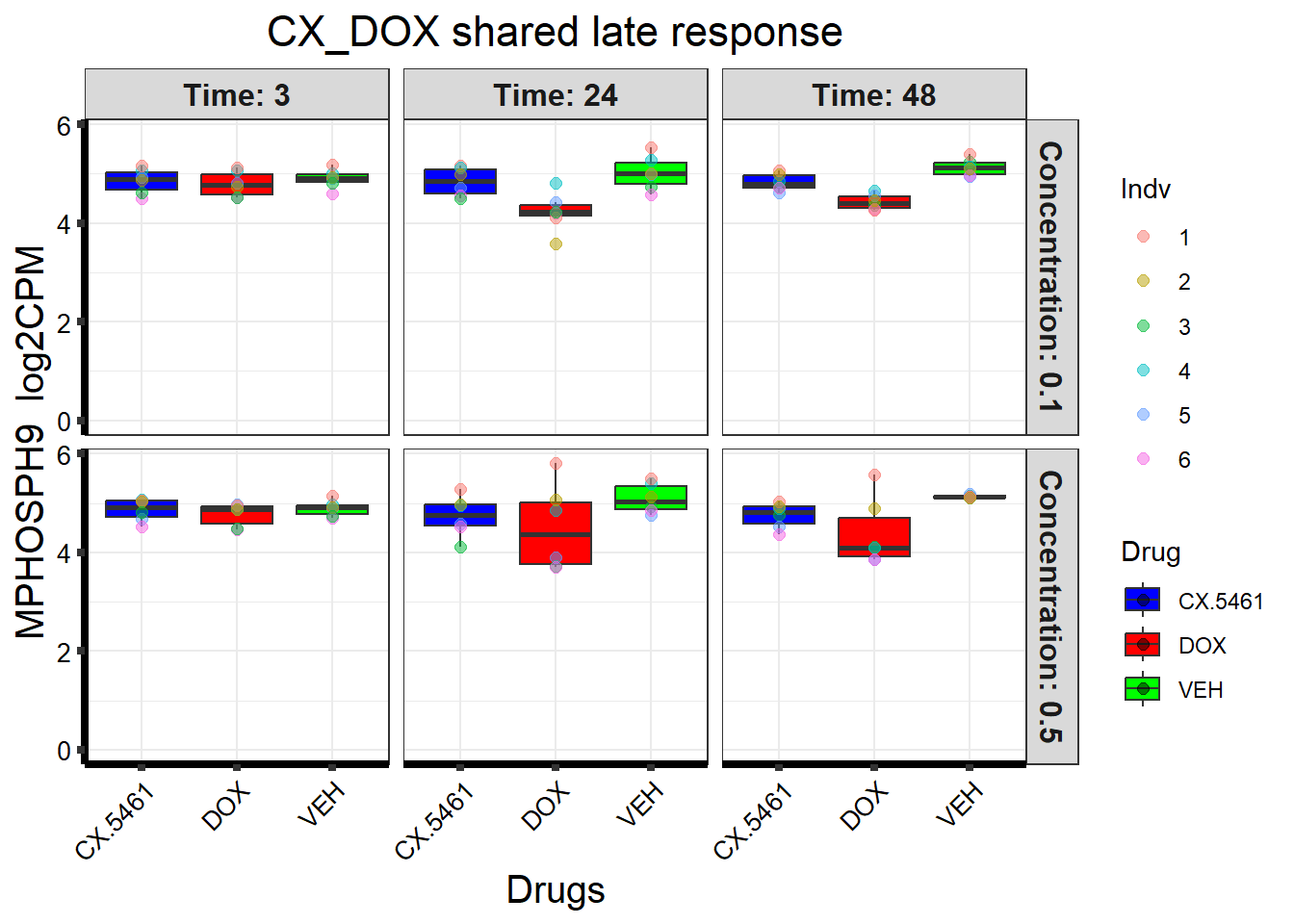
📌 CX_DOX shared late response (MPHOSPH9)
# Load the dataset from the data folder
# Load the dataset from the data folder

# Filter data for the gene with Entrez ID: 10198
gene_data <- boxplot1[boxplot1$ENTREZID == 10198, ]

# Check if gene_data is empty
if(nrow(gene_data) == 0) {
  stop("No data found for the selected gene ENTIREZID 10198.")
}

# Reshape data from wide to long format
gene_data_long <- melt(gene_data,
                       id.vars = c("ENTREZID", "SYMBOL", "GENENAME"),
                       variable.name = "Sample",
                       value.name = "log2CPM")

# Print some sample names for debugging
print(unique(gene_data_long$Sample))
[1] 17.3_CX.5461_0.1_3 17.3_DOX_0.5_24
[4] 87.1_DOX_0.5_24 87.1_VEH_0.1_24 87.1_VEH_0.5_24
[7] 87.1_CX.5461_0.1_48 87.1_CX.5461_0.5_48 87.1_DOX_0.1_48
[10] 87.1_DOX_0.5_48 87.1_VEH_0.1_48 87.1_VEH_0.5_48
[13] 17.3_VEH_0.1_24 17.3_VEH_0.5_24 17.3_CX.5461_0.1_48
[16] 17.3_CX.5461_0.5_48 17.3_DOX_0.1_48 17.3_DOX_0.5_48
[19] 17.3_VEH_0.1_48 17.3_VEH_0.5_48 84.1_CX.5461_0.1_3
[22] 17.3_CX.5461_0.5_3 84.1_CX.5461_0.5_3 84.1_DOX_0.1_3
[25] 84.1_DOX_0.5_3 84.1_VEH_0.1_3 84.1_VEH_0.5_3
[28] 84.1_CX.5461_0.1_24 84.1_CX.5461_0.5_24 84.1_DOX_0.1_24
[31] 84.1_DOX_0.5_24 84.1_VEH_0.1_24 17.3_DOX_0.1_3
[34] 84.1_VEH_0.5_24 84.1_CX.5461_0.1_48 84.1_CX.5461_0.5_48
[37] 84.1_DOX_0.1_48 84.1_DOX_0.5_48 84.1_VEH_0.1_48
[40] 84.1_VEH_0.5_48 90.1_CX.5461_0.1_3 90.1_CX.5461_0.5_3
[43] 90.1_DOX_0.1_3 17.3_DOX_0.5_3 90.1_DOX_0.5_3
[46] 90.1_VEH_0.1_3 90.1_VEH_0.5_3 90.1_CX.5461_0.1_24
[49] 90.1_CX.5461_0.5_24 90.1_DOX_0.1_24 90.1_DOX_0.5_24
[52] 90.1_VEH_0.1_24 90.1_VEH_0.5_24 90.1_CX.5461_0.1_48
[55] 17.3_VEH_0.1_3 90.1_CX.5461_0.5_48 90.1_DOX_0.1_48
[58] 90.1_DOX_0.5_48 90.1_VEH_0.1_48 90.1_VEH_0.5_48
[61] 75.1_CX.5461_0.1_3 75.1_CX.5461_0.5_3 75.1_DOX_0.1_3
[64] 75.1_DOX_0.5_3 75.1_VEH_0.1_3 17.3_VEH_0.5_3
[67] 75.1_VEH_0.5_3 75.1_CX.5461_0.1_24 75.1_CX.5461_0.5_24
[70] 75.1_DOX_0.1_24 75.1_DOX_0.5_24 75.1_VEH_0.1_24
[73] 75.1_VEH_0.5_24 75.1_CX.5461_0.1_48 75.1_CX.5461_0.5_48
[76] 75.1_DOX_0.1_48 17.3_CX.5461_0.1_24 75.1_DOX_0.5_48
[79] 75.1_VEH_0.1_48 75.1_VEH_0.5_48 78.1_CX.5461_0.1_3
[82] 78.1_CX.5461_0.5_3 78.1_DOX_0.1_3 78.1_DOX_0.5_3
[85] 78.1_VEH_0.1_3 78.1_VEH_0.5_3 78.1_CX.5461_0.1_24
[88] 17.3_CX.5461_0.5_24 78.1_CX.5461_0.5_24 78.1_DOX_0.1_24
[91] 78.1_DOX_0.5_24 78.1_VEH_0.1_24 78.1_VEH_0.5_24
[94] 78.1_CX.5461_0.1_48 78.1_CX.5461_0.5_48 78.1_DOX_0.1_48
[97] 78.1_DOX_0.5_48 78.1_VEH_0.1_48 17.3_DOX_0.1_24
[100] 78.1_VEH_0.5_48 87.1_CX.5461_0.1_3 87.1_CX.5461_0.5_3
[103] 87.1_DOX_0.1_3 87.1_DOX_0.5_3 87.1_VEH_0.1_3
[106] 87.1_VEH_0.5_3 87.1_CX.5461_0.1_24 87.1_CX.5461_0.5_24
[109] 87.1_DOX_0.1_24
109 Levels: 17.3_CX.5461_0.1_3 17.3_DOX_0.5_24 ... 87.1_DOX_0.1_24# Extract details from sample names
gene_data_long <- gene_data_long %>%
mutate(
Time = sub(".*_(\\d+)$", "\\1", Sample),
Concentration = sub(".*_(0\\.\\d)_\\d+$", "\\1", Sample),
Drug = sub(".*_(CX\\.5461|DOX|VEH)_.*", "\\1", Sample),
Indv = sub("^([0-9]+\\.[0-9]+)_.*", "\\1", Sample) # Ensure correct pattern extraction
)
# Print extracted `Indv` column for debugging
print(unique(gene_data_long$Indv))[1] "" "17.3" "87.1" "84.1" "90.1" "75.1" "78.1"# Convert extracted columns to factors
gene_data_long$Time <- factor(gene_data_long$Time, levels = c("3", "24", "48"))
gene_data_long$Concentration <- factor(gene_data_long$Concentration, levels = c("0.1", "0.5"))
# Ensure each concentration facet only shows relevant data
gene_data_long <- gene_data_long %>%
group_by(Concentration) %>%
filter(all(Concentration == "0.1") | all(Concentration == "0.5")) %>%
ungroup()
# Map individual IDs
indv_mapping <- c("75.1" = "1", "78.1" = "2", "87.1" = "3", "17.3" = "4", "84.1" = "5", "90.1" = "6")
# Ensure `Indv` values match the keys in `indv_mapping`
gene_data_long <- gene_data_long %>%
mutate(
Indv = ifelse(Indv %in% names(indv_mapping), indv_mapping[Indv], NA)
)
# Print `Indv` column again to confirm mapping worked
print(unique(gene_data_long$Indv))[1] "4" "3" "5" "6" "1" "2"# Check for missing values and handle them
gene_data_long <- gene_data_long %>%
mutate(Indv = ifelse(is.na(Indv), "Unknown", Indv)) # Assign "Unknown" to unidentified individuals
# Define drug colors
drug_palette <- c("CX.5461" = "blue", "DOX" = "red", "VEH" = "green")
# Extract the gene symbol for labeling
gene_symbol <- unique(gene_data_long$SYMBOL)[1]
# Create the boxplot
ggplot(gene_data_long, aes(x = Drug, y = log2CPM, fill = Drug)) +
geom_boxplot(outlier.shape = NA) +
scale_fill_manual(values = drug_palette) +
facet_grid(Concentration ~ Time, labeller = label_both) +
geom_point(aes(color = Indv), size = 2, alpha = 0.5,
position = position_jitter(width = -0.3, height = 0)) +
ggtitle("CX_DOX shared late response") +
labs(
title = "CX_DOX shared late response",
x = "Drugs",
y = paste(gene_symbol, " log2CPM")
) +
ylim(0, NA) +
theme_bw() +
theme(
plot.title = element_text(size = rel(1.5), hjust = 0.5),
axis.title = element_text(size = 15, color = "black"),
axis.ticks = element_line(linewidth = 1.5),
axis.line = element_line(linewidth = 1.5),
axis.text.y = element_text(size = 10, color = "black"),
axis.text.x = element_text(size = 10, color = "black", angle = 45, hjust = 1),
strip.text = element_text(size = 12, face = "bold")
)
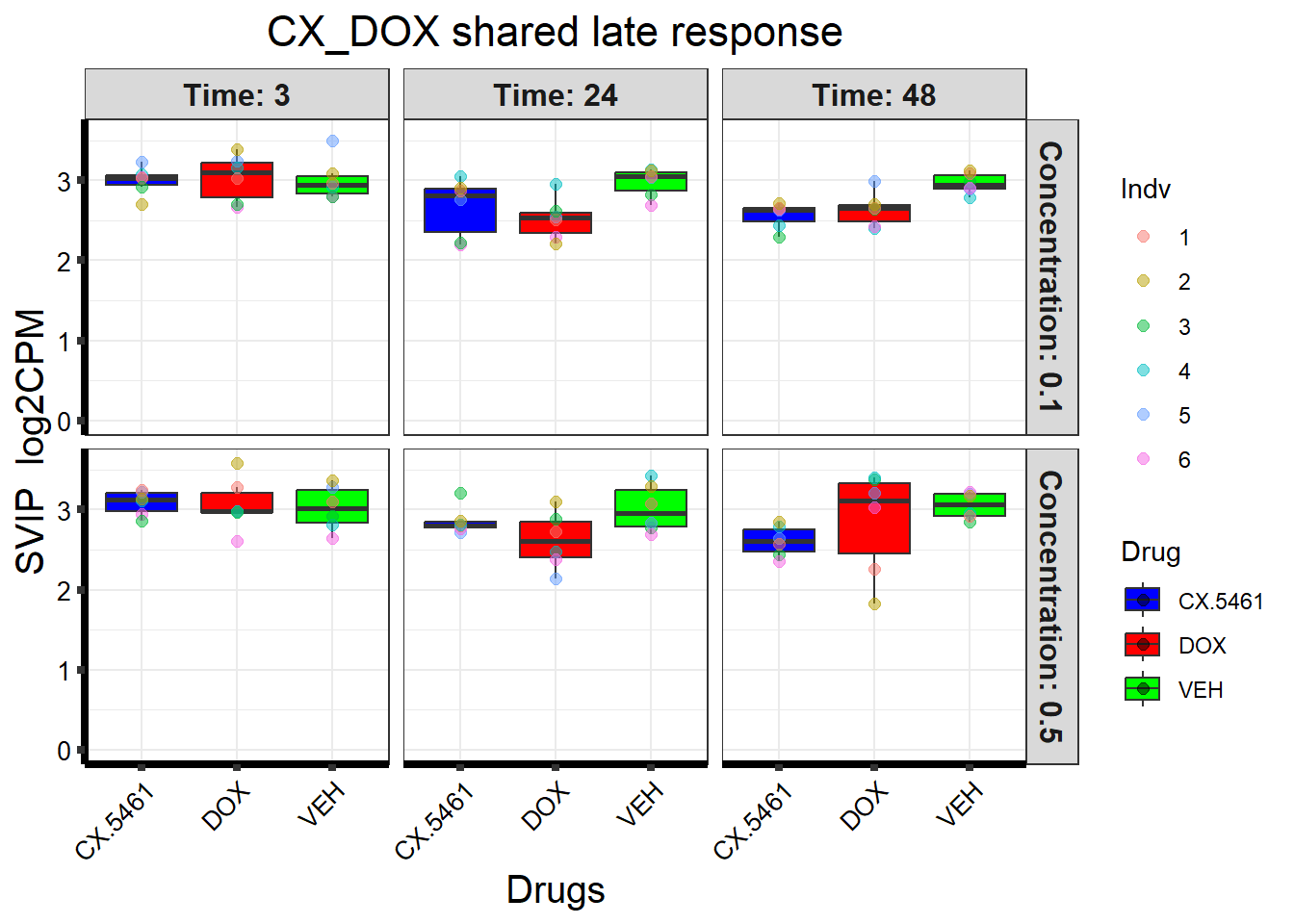
📌 CX_DOX shared late response (SVIP)
# Load the dataset from the data folder
# Load the dataset from the data folder

# Filter data for the gene with Entrez ID: 258010
gene_data <- boxplot1[boxplot1$ENTREZID == 258010, ]

# Check if gene_data is empty
if(nrow(gene_data) == 0) {
  stop("No data found for the selected gene ENTIREZID 258010.")
}

# Reshape data from wide to long format
gene_data_long <- melt(gene_data,
                       id.vars = c("ENTREZID", "SYMBOL", "GENENAME"),
                       variable.name = "Sample",
                       value.name = "log2CPM")

# Print some sample names for debugging
print(unique(gene_data_long$Sample))
[1] 17.3_CX.5461_0.1_3 17.3_DOX_0.5_24
[4] 87.1_DOX_0.5_24 87.1_VEH_0.1_24 87.1_VEH_0.5_24
[7] 87.1_CX.5461_0.1_48 87.1_CX.5461_0.5_48 87.1_DOX_0.1_48
[10] 87.1_DOX_0.5_48 87.1_VEH_0.1_48 87.1_VEH_0.5_48
[13] 17.3_VEH_0.1_24 17.3_VEH_0.5_24 17.3_CX.5461_0.1_48
[16] 17.3_CX.5461_0.5_48 17.3_DOX_0.1_48 17.3_DOX_0.5_48
[19] 17.3_VEH_0.1_48 17.3_VEH_0.5_48 84.1_CX.5461_0.1_3
[22] 17.3_CX.5461_0.5_3 84.1_CX.5461_0.5_3 84.1_DOX_0.1_3
[25] 84.1_DOX_0.5_3 84.1_VEH_0.1_3 84.1_VEH_0.5_3
[28] 84.1_CX.5461_0.1_24 84.1_CX.5461_0.5_24 84.1_DOX_0.1_24
[31] 84.1_DOX_0.5_24 84.1_VEH_0.1_24 17.3_DOX_0.1_3
[34] 84.1_VEH_0.5_24 84.1_CX.5461_0.1_48 84.1_CX.5461_0.5_48
[37] 84.1_DOX_0.1_48 84.1_DOX_0.5_48 84.1_VEH_0.1_48
[40] 84.1_VEH_0.5_48 90.1_CX.5461_0.1_3 90.1_CX.5461_0.5_3
[43] 90.1_DOX_0.1_3 17.3_DOX_0.5_3 90.1_DOX_0.5_3
[46] 90.1_VEH_0.1_3 90.1_VEH_0.5_3 90.1_CX.5461_0.1_24
[49] 90.1_CX.5461_0.5_24 90.1_DOX_0.1_24 90.1_DOX_0.5_24
[52] 90.1_VEH_0.1_24 90.1_VEH_0.5_24 90.1_CX.5461_0.1_48
[55] 17.3_VEH_0.1_3 90.1_CX.5461_0.5_48 90.1_DOX_0.1_48
[58] 90.1_DOX_0.5_48 90.1_VEH_0.1_48 90.1_VEH_0.5_48
[61] 75.1_CX.5461_0.1_3 75.1_CX.5461_0.5_3 75.1_DOX_0.1_3
[64] 75.1_DOX_0.5_3 75.1_VEH_0.1_3 17.3_VEH_0.5_3
[67] 75.1_VEH_0.5_3 75.1_CX.5461_0.1_24 75.1_CX.5461_0.5_24
[70] 75.1_DOX_0.1_24 75.1_DOX_0.5_24 75.1_VEH_0.1_24
[73] 75.1_VEH_0.5_24 75.1_CX.5461_0.1_48 75.1_CX.5461_0.5_48
[76] 75.1_DOX_0.1_48 17.3_CX.5461_0.1_24 75.1_DOX_0.5_48
[79] 75.1_VEH_0.1_48 75.1_VEH_0.5_48 78.1_CX.5461_0.1_3
[82] 78.1_CX.5461_0.5_3 78.1_DOX_0.1_3 78.1_DOX_0.5_3
[85] 78.1_VEH_0.1_3 78.1_VEH_0.5_3 78.1_CX.5461_0.1_24
[88] 17.3_CX.5461_0.5_24 78.1_CX.5461_0.5_24 78.1_DOX_0.1_24
[91] 78.1_DOX_0.5_24 78.1_VEH_0.1_24 78.1_VEH_0.5_24
[94] 78.1_CX.5461_0.1_48 78.1_CX.5461_0.5_48 78.1_DOX_0.1_48
[97] 78.1_DOX_0.5_48 78.1_VEH_0.1_48 17.3_DOX_0.1_24
[100] 78.1_VEH_0.5_48 87.1_CX.5461_0.1_3 87.1_CX.5461_0.5_3
[103] 87.1_DOX_0.1_3 87.1_DOX_0.5_3 87.1_VEH_0.1_3
[106] 87.1_VEH_0.5_3 87.1_CX.5461_0.1_24 87.1_CX.5461_0.5_24
[109] 87.1_DOX_0.1_24
109 Levels: 17.3_CX.5461_0.1_3 17.3_DOX_0.5_24 ... 87.1_DOX_0.1_24# Extract details from sample names
gene_data_long <- gene_data_long %>%
mutate(
Time = sub(".*_(\\d+)$", "\\1", Sample),
Concentration = sub(".*_(0\\.\\d)_\\d+$", "\\1", Sample),
Drug = sub(".*_(CX\\.5461|DOX|VEH)_.*", "\\1", Sample),
Indv = sub("^([0-9]+\\.[0-9]+)_.*", "\\1", Sample) # Ensure correct pattern extraction
)
# Print extracted `Indv` column for debugging
print(unique(gene_data_long$Indv))[1] "" "17.3" "87.1" "84.1" "90.1" "75.1" "78.1"# Convert extracted columns to factors
gene_data_long$Time <- factor(gene_data_long$Time, levels = c("3", "24", "48"))
gene_data_long$Concentration <- factor(gene_data_long$Concentration, levels = c("0.1", "0.5"))
# Ensure each concentration facet only shows relevant data
gene_data_long <- gene_data_long %>%
group_by(Concentration) %>%
filter(all(Concentration == "0.1") | all(Concentration == "0.5")) %>%
ungroup()
# Map individual IDs
indv_mapping <- c("75.1" = "1", "78.1" = "2", "87.1" = "3", "17.3" = "4", "84.1" = "5", "90.1" = "6")
# Ensure `Indv` values match the keys in `indv_mapping`
gene_data_long <- gene_data_long %>%
mutate(
Indv = ifelse(Indv %in% names(indv_mapping), indv_mapping[Indv], NA)
)
# Print `Indv` column again to confirm mapping worked
print(unique(gene_data_long$Indv))[1] "4" "3" "5" "6" "1" "2"# Check for missing values and handle them
gene_data_long <- gene_data_long %>%
mutate(Indv = ifelse(is.na(Indv), "Unknown", Indv)) # Assign "Unknown" to unidentified individuals
# Define drug colors
drug_palette <- c("CX.5461" = "blue", "DOX" = "red", "VEH" = "green")
# Extract the gene symbol for labeling
gene_symbol <- unique(gene_data_long$SYMBOL)[1]
# Create the boxplot
ggplot(gene_data_long, aes(x = Drug, y = log2CPM, fill = Drug)) +
geom_boxplot(outlier.shape = NA) +
scale_fill_manual(values = drug_palette) +
facet_grid(Concentration ~ Time, labeller = label_both) +
geom_point(aes(color = Indv), size = 2, alpha = 0.5,
position = position_jitter(width = -0.3, height = 0)) +
ggtitle("CX_DOX shared late response") +
labs(
title = "CX_DOX shared late response",
x = "Drugs",
y = paste(gene_symbol, " log2CPM")
) +
ylim(0, NA) +
theme_bw() +
theme(
plot.title = element_text(size = rel(1.5), hjust = 0.5),
axis.title = element_text(size = 15, color = "black"),
axis.ticks = element_line(linewidth = 1.5),
axis.line = element_line(linewidth = 1.5),
axis.text.y = element_text(size = 10, color = "black"),
axis.text.x = element_text(size = 10, color = "black", angle = 45, hjust = 1),
strip.text = element_text(size = 12, face = "bold")
)
| Version | Author | Date |
|---|---|---|
| ebfddcd | sayanpaul01 | 2025-02-23 |
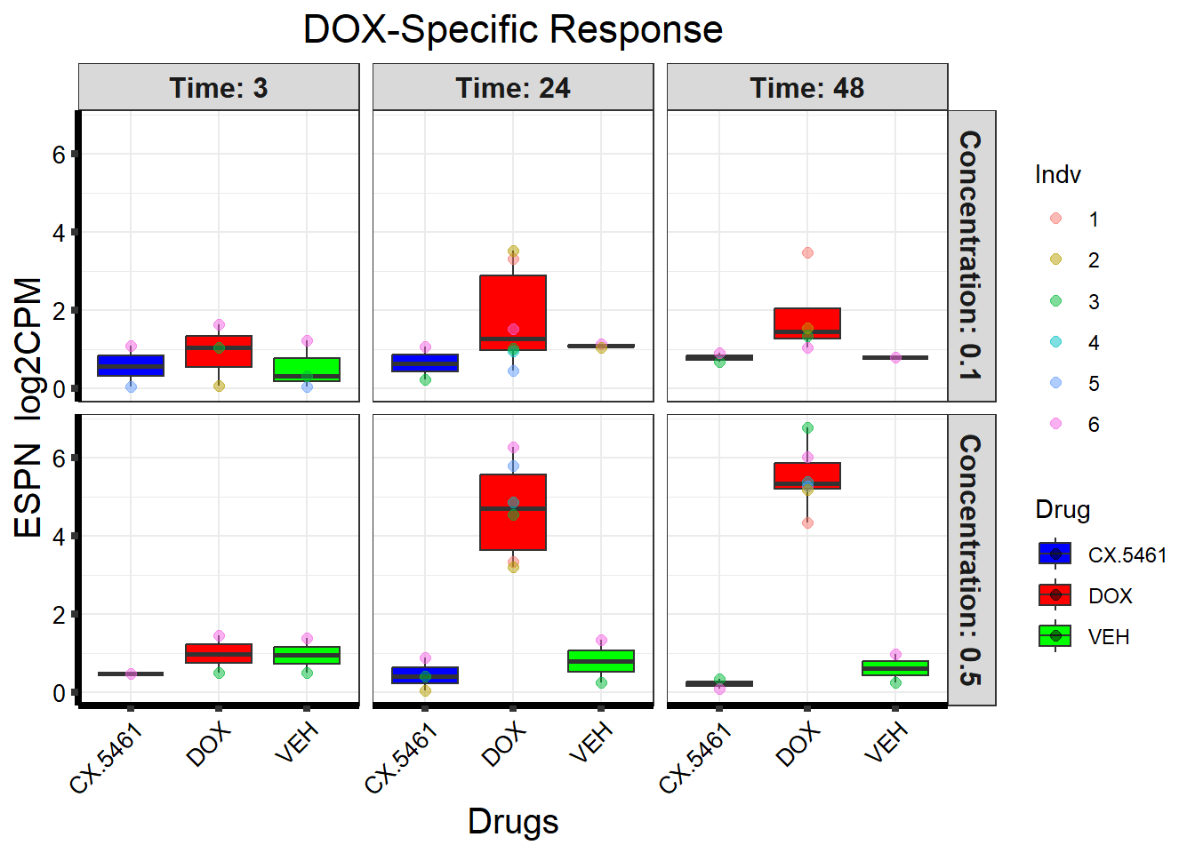
📌 DOX-Specific Response (ESPN)
# Load the dataset from the data folder
# Load the dataset from the data folder

# Filter data for the gene with Entrez ID:  83715
gene_data <- boxplot1[boxplot1$ENTREZID ==  83715, ]

# Check if gene_data is empty
if(nrow(gene_data) == 0) {
  stop("No data found for the selected gene ENTIREZID
83715.")
}

# Reshape data from wide to long format
gene_data_long <- melt(gene_data,
                       id.vars = c("ENTREZID", "SYMBOL", "GENENAME"),
                       variable.name = "Sample",
                       value.name = "log2CPM")

# Print some sample names for debugging
print(unique(gene_data_long$Sample))
[1] 17.3_CX.5461_0.1_3 17.3_DOX_0.5_24
[4] 87.1_DOX_0.5_24 87.1_VEH_0.1_24 87.1_VEH_0.5_24
[7] 87.1_CX.5461_0.1_48 87.1_CX.5461_0.5_48 87.1_DOX_0.1_48
[10] 87.1_DOX_0.5_48 87.1_VEH_0.1_48 87.1_VEH_0.5_48
[13] 17.3_VEH_0.1_24 17.3_VEH_0.5_24 17.3_CX.5461_0.1_48
[16] 17.3_CX.5461_0.5_48 17.3_DOX_0.1_48 17.3_DOX_0.5_48
[19] 17.3_VEH_0.1_48 17.3_VEH_0.5_48 84.1_CX.5461_0.1_3
[22] 17.3_CX.5461_0.5_3 84.1_CX.5461_0.5_3 84.1_DOX_0.1_3
[25] 84.1_DOX_0.5_3 84.1_VEH_0.1_3 84.1_VEH_0.5_3
[28] 84.1_CX.5461_0.1_24 84.1_CX.5461_0.5_24 84.1_DOX_0.1_24
[31] 84.1_DOX_0.5_24 84.1_VEH_0.1_24 17.3_DOX_0.1_3
[34] 84.1_VEH_0.5_24 84.1_CX.5461_0.1_48 84.1_CX.5461_0.5_48
[37] 84.1_DOX_0.1_48 84.1_DOX_0.5_48 84.1_VEH_0.1_48
[40] 84.1_VEH_0.5_48 90.1_CX.5461_0.1_3 90.1_CX.5461_0.5_3
[43] 90.1_DOX_0.1_3 17.3_DOX_0.5_3 90.1_DOX_0.5_3
[46] 90.1_VEH_0.1_3 90.1_VEH_0.5_3 90.1_CX.5461_0.1_24
[49] 90.1_CX.5461_0.5_24 90.1_DOX_0.1_24 90.1_DOX_0.5_24
[52] 90.1_VEH_0.1_24 90.1_VEH_0.5_24 90.1_CX.5461_0.1_48
[55] 17.3_VEH_0.1_3 90.1_CX.5461_0.5_48 90.1_DOX_0.1_48
[58] 90.1_DOX_0.5_48 90.1_VEH_0.1_48 90.1_VEH_0.5_48
[61] 75.1_CX.5461_0.1_3 75.1_CX.5461_0.5_3 75.1_DOX_0.1_3
[64] 75.1_DOX_0.5_3 75.1_VEH_0.1_3 17.3_VEH_0.5_3
[67] 75.1_VEH_0.5_3 75.1_CX.5461_0.1_24 75.1_CX.5461_0.5_24
[70] 75.1_DOX_0.1_24 75.1_DOX_0.5_24 75.1_VEH_0.1_24
[73] 75.1_VEH_0.5_24 75.1_CX.5461_0.1_48 75.1_CX.5461_0.5_48
[76] 75.1_DOX_0.1_48 17.3_CX.5461_0.1_24 75.1_DOX_0.5_48
[79] 75.1_VEH_0.1_48 75.1_VEH_0.5_48 78.1_CX.5461_0.1_3
[82] 78.1_CX.5461_0.5_3 78.1_DOX_0.1_3 78.1_DOX_0.5_3
[85] 78.1_VEH_0.1_3 78.1_VEH_0.5_3 78.1_CX.5461_0.1_24
[88] 17.3_CX.5461_0.5_24 78.1_CX.5461_0.5_24 78.1_DOX_0.1_24
[91] 78.1_DOX_0.5_24 78.1_VEH_0.1_24 78.1_VEH_0.5_24
[94] 78.1_CX.5461_0.1_48 78.1_CX.5461_0.5_48 78.1_DOX_0.1_48
[97] 78.1_DOX_0.5_48 78.1_VEH_0.1_48 17.3_DOX_0.1_24
[100] 78.1_VEH_0.5_48 87.1_CX.5461_0.1_3 87.1_CX.5461_0.5_3
[103] 87.1_DOX_0.1_3 87.1_DOX_0.5_3 87.1_VEH_0.1_3
[106] 87.1_VEH_0.5_3 87.1_CX.5461_0.1_24 87.1_CX.5461_0.5_24
[109] 87.1_DOX_0.1_24
109 Levels: 17.3_CX.5461_0.1_3 17.3_DOX_0.5_24 ... 87.1_DOX_0.1_24# Extract details from sample names
gene_data_long <- gene_data_long %>%
mutate(
Time = sub(".*_(\\d+)$", "\\1", Sample),
Concentration = sub(".*_(0\\.\\d)_\\d+$", "\\1", Sample),
Drug = sub(".*_(CX\\.5461|DOX|VEH)_.*", "\\1", Sample),
Indv = sub("^([0-9]+\\.[0-9]+)_.*", "\\1", Sample) # Ensure correct pattern extraction
)
# Print extracted `Indv` column for debugging
print(unique(gene_data_long$Indv))[1] "" "17.3" "87.1" "84.1" "90.1" "75.1" "78.1"# Convert extracted columns to factors
gene_data_long$Time <- factor(gene_data_long$Time, levels = c("3", "24", "48"))
gene_data_long$Concentration <- factor(gene_data_long$Concentration, levels = c("0.1", "0.5"))
# Ensure each concentration facet only shows relevant data
gene_data_long <- gene_data_long %>%
group_by(Concentration) %>%
filter(all(Concentration == "0.1") | all(Concentration == "0.5")) %>%
ungroup()
# Map individual IDs
indv_mapping <- c("75.1" = "1", "78.1" = "2", "87.1" = "3", "17.3" = "4", "84.1" = "5", "90.1" = "6")
# Ensure `Indv` values match the keys in `indv_mapping`
gene_data_long <- gene_data_long %>%
mutate(
Indv = ifelse(Indv %in% names(indv_mapping), indv_mapping[Indv], NA)
)
# Print `Indv` column again to confirm mapping worked
print(unique(gene_data_long$Indv))[1] "4" "3" "5" "6" "1" "2"# Check for missing values and handle them
gene_data_long <- gene_data_long %>%
mutate(Indv = ifelse(is.na(Indv), "Unknown", Indv)) # Assign "Unknown" to unidentified individuals
# Define drug colors
drug_palette <- c("CX.5461" = "blue", "DOX" = "red", "VEH" = "green")
# Extract the gene symbol for labeling
gene_symbol <- unique(gene_data_long$SYMBOL)[1]
# Create the boxplot
ggplot(gene_data_long, aes(x = Drug, y = log2CPM, fill = Drug)) +
geom_boxplot(outlier.shape = NA) +
scale_fill_manual(values = drug_palette) +
facet_grid(Concentration ~ Time, labeller = label_both) +
geom_point(aes(color = Indv), size = 2, alpha = 0.5,
position = position_jitter(width = -0.3, height = 0)) +
ggtitle("DOX-Specific Response") +
labs(
title = "DOX-Specific Response",
x = "Drugs",
y = paste(gene_symbol, " log2CPM")
) +
ylim(0, NA) +
theme_bw() +
theme(
plot.title = element_text(size = rel(1.5), hjust = 0.5),
axis.title = element_text(size = 15, color = "black"),
axis.ticks = element_line(linewidth = 1.5),
axis.line = element_line(linewidth = 1.5),
axis.text.y = element_text(size = 10, color = "black"),
axis.text.x = element_text(size = 10, color = "black", angle = 45, hjust = 1),
strip.text = element_text(size = 12, face = "bold")
)
| Version | Author | Date |
|---|---|---|
| ebfddcd | sayanpaul01 | 2025-02-23 |
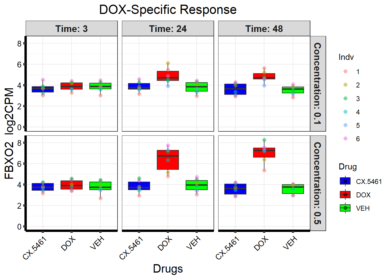
📌 DOX-Specific Response (FBXO2)
# Load the dataset from the data folder
# Load the dataset from the data folder

# Filter data for the gene with Entrez ID:  26232
gene_data <- boxplot1[boxplot1$ENTREZID ==  26232, ]

# Check if gene_data is empty
if(nrow(gene_data) == 0) {
  stop("No data found for the selected gene ENTIREZID
26232.")
}

# Reshape data from wide to long format
gene_data_long <- melt(gene_data,
                       id.vars = c("ENTREZID", "SYMBOL", "GENENAME"),
                       variable.name = "Sample",
                       value.name = "log2CPM")

# Print some sample names for debugging
print(unique(gene_data_long$Sample))
[1] 17.3_CX.5461_0.1_3 17.3_DOX_0.5_24
[4] 87.1_DOX_0.5_24 87.1_VEH_0.1_24 87.1_VEH_0.5_24
[7] 87.1_CX.5461_0.1_48 87.1_CX.5461_0.5_48 87.1_DOX_0.1_48
[10] 87.1_DOX_0.5_48 87.1_VEH_0.1_48 87.1_VEH_0.5_48
[13] 17.3_VEH_0.1_24 17.3_VEH_0.5_24 17.3_CX.5461_0.1_48
[16] 17.3_CX.5461_0.5_48 17.3_DOX_0.1_48 17.3_DOX_0.5_48
[19] 17.3_VEH_0.1_48 17.3_VEH_0.5_48 84.1_CX.5461_0.1_3
[22] 17.3_CX.5461_0.5_3 84.1_CX.5461_0.5_3 84.1_DOX_0.1_3
[25] 84.1_DOX_0.5_3 84.1_VEH_0.1_3 84.1_VEH_0.5_3
[28] 84.1_CX.5461_0.1_24 84.1_CX.5461_0.5_24 84.1_DOX_0.1_24
[31] 84.1_DOX_0.5_24 84.1_VEH_0.1_24 17.3_DOX_0.1_3
[34] 84.1_VEH_0.5_24 84.1_CX.5461_0.1_48 84.1_CX.5461_0.5_48
[37] 84.1_DOX_0.1_48 84.1_DOX_0.5_48 84.1_VEH_0.1_48
[40] 84.1_VEH_0.5_48 90.1_CX.5461_0.1_3 90.1_CX.5461_0.5_3
[43] 90.1_DOX_0.1_3 17.3_DOX_0.5_3 90.1_DOX_0.5_3
[46] 90.1_VEH_0.1_3 90.1_VEH_0.5_3 90.1_CX.5461_0.1_24
[49] 90.1_CX.5461_0.5_24 90.1_DOX_0.1_24 90.1_DOX_0.5_24
[52] 90.1_VEH_0.1_24 90.1_VEH_0.5_24 90.1_CX.5461_0.1_48
[55] 17.3_VEH_0.1_3 90.1_CX.5461_0.5_48 90.1_DOX_0.1_48
[58] 90.1_DOX_0.5_48 90.1_VEH_0.1_48 90.1_VEH_0.5_48
[61] 75.1_CX.5461_0.1_3 75.1_CX.5461_0.5_3 75.1_DOX_0.1_3
[64] 75.1_DOX_0.5_3 75.1_VEH_0.1_3 17.3_VEH_0.5_3
[67] 75.1_VEH_0.5_3 75.1_CX.5461_0.1_24 75.1_CX.5461_0.5_24
[70] 75.1_DOX_0.1_24 75.1_DOX_0.5_24 75.1_VEH_0.1_24
[73] 75.1_VEH_0.5_24 75.1_CX.5461_0.1_48 75.1_CX.5461_0.5_48
[76] 75.1_DOX_0.1_48 17.3_CX.5461_0.1_24 75.1_DOX_0.5_48
[79] 75.1_VEH_0.1_48 75.1_VEH_0.5_48 78.1_CX.5461_0.1_3
[82] 78.1_CX.5461_0.5_3 78.1_DOX_0.1_3 78.1_DOX_0.5_3
[85] 78.1_VEH_0.1_3 78.1_VEH_0.5_3 78.1_CX.5461_0.1_24
[88] 17.3_CX.5461_0.5_24 78.1_CX.5461_0.5_24 78.1_DOX_0.1_24
[91] 78.1_DOX_0.5_24 78.1_VEH_0.1_24 78.1_VEH_0.5_24
[94] 78.1_CX.5461_0.1_48 78.1_CX.5461_0.5_48 78.1_DOX_0.1_48
[97] 78.1_DOX_0.5_48 78.1_VEH_0.1_48 17.3_DOX_0.1_24
[100] 78.1_VEH_0.5_48 87.1_CX.5461_0.1_3 87.1_CX.5461_0.5_3
[103] 87.1_DOX_0.1_3 87.1_DOX_0.5_3 87.1_VEH_0.1_3
[106] 87.1_VEH_0.5_3 87.1_CX.5461_0.1_24 87.1_CX.5461_0.5_24
[109] 87.1_DOX_0.1_24
109 Levels: 17.3_CX.5461_0.1_3 17.3_DOX_0.5_24 ... 87.1_DOX_0.1_24# Extract details from sample names
gene_data_long <- gene_data_long %>%
mutate(
Time = sub(".*_(\\d+)$", "\\1", Sample),
Concentration = sub(".*_(0\\.\\d)_\\d+$", "\\1", Sample),
Drug = sub(".*_(CX\\.5461|DOX|VEH)_.*", "\\1", Sample),
Indv = sub("^([0-9]+\\.[0-9]+)_.*", "\\1", Sample) # Ensure correct pattern extraction
)
# Print extracted `Indv` column for debugging
print(unique(gene_data_long$Indv))[1] "" "17.3" "87.1" "84.1" "90.1" "75.1" "78.1"# Convert extracted columns to factors
gene_data_long$Time <- factor(gene_data_long$Time, levels = c("3", "24", "48"))
gene_data_long$Concentration <- factor(gene_data_long$Concentration, levels = c("0.1", "0.5"))
# Ensure each concentration facet only shows relevant data
gene_data_long <- gene_data_long %>%
group_by(Concentration) %>%
filter(all(Concentration == "0.1") | all(Concentration == "0.5")) %>%
ungroup()
# Map individual IDs
indv_mapping <- c("75.1" = "1", "78.1" = "2", "87.1" = "3", "17.3" = "4", "84.1" = "5", "90.1" = "6")
# Ensure `Indv` values match the keys in `indv_mapping`
gene_data_long <- gene_data_long %>%
mutate(
Indv = ifelse(Indv %in% names(indv_mapping), indv_mapping[Indv], NA)
)
# Print `Indv` column again to confirm mapping worked
print(unique(gene_data_long$Indv))[1] "4" "3" "5" "6" "1" "2"# Check for missing values and handle them
gene_data_long <- gene_data_long %>%
mutate(Indv = ifelse(is.na(Indv), "Unknown", Indv)) # Assign "Unknown" to unidentified individuals
# Define drug colors
drug_palette <- c("CX.5461" = "blue", "DOX" = "red", "VEH" = "green")
# Extract the gene symbol for labeling
gene_symbol <- unique(gene_data_long$SYMBOL)[1]
# Create the boxplot
ggplot(gene_data_long, aes(x = Drug, y = log2CPM, fill = Drug)) +
geom_boxplot(outlier.shape = NA) +
scale_fill_manual(values = drug_palette) +
facet_grid(Concentration ~ Time, labeller = label_both) +
geom_point(aes(color = Indv), size = 2, alpha = 0.5,
position = position_jitter(width = -0.3, height = 0)) +
ggtitle("DOX-Specific Response") +
labs(
title = "DOX-Specific Response",
x = "Drugs",
y = paste(gene_symbol, " log2CPM")
) +
ylim(0, NA) +
theme_bw() +
theme(
plot.title = element_text(size = rel(1.5), hjust = 0.5),
axis.title = element_text(size = 15, color = "black"),
axis.ticks = element_line(linewidth = 1.5),
axis.line = element_line(linewidth = 1.5),
axis.text.y = element_text(size = 10, color = "black"),
axis.text.x = element_text(size = 10, color = "black", angle = 45, hjust = 1),
strip.text = element_text(size = 12, face = "bold")
)
| Version | Author | Date |
|---|---|---|
| ebfddcd | sayanpaul01 | 2025-02-23 |
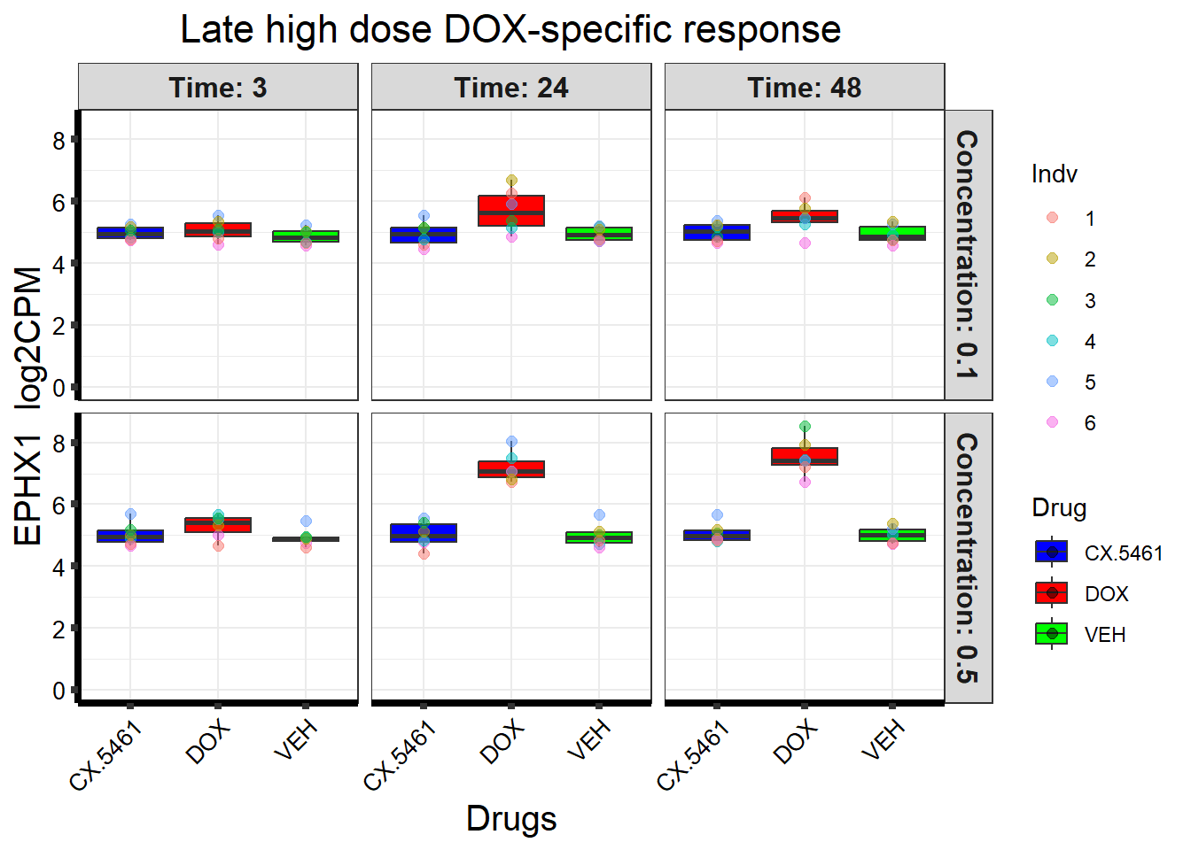
📌 Late high dose DOX-specific response (EPHX1)
# Load the dataset from the data folder
# Load the dataset from the data folder

# Filter data for the gene with Entrez ID:  2052
gene_data <- boxplot1[boxplot1$ENTREZID ==  2052, ]

# Check if gene_data is empty
if(nrow(gene_data) == 0) {
  stop("No data found for the selected gene ENTIREZID
2052.")
}

# Reshape data from wide to long format
gene_data_long <- melt(gene_data,
                       id.vars = c("ENTREZID", "SYMBOL", "GENENAME"),
                       variable.name = "Sample",
                       value.name = "log2CPM")

# Print some sample names for debugging
print(unique(gene_data_long$Sample))
[1] 17.3_CX.5461_0.1_3 17.3_DOX_0.5_24
[4] 87.1_DOX_0.5_24 87.1_VEH_0.1_24 87.1_VEH_0.5_24
[7] 87.1_CX.5461_0.1_48 87.1_CX.5461_0.5_48 87.1_DOX_0.1_48
[10] 87.1_DOX_0.5_48 87.1_VEH_0.1_48 87.1_VEH_0.5_48
[13] 17.3_VEH_0.1_24 17.3_VEH_0.5_24 17.3_CX.5461_0.1_48
[16] 17.3_CX.5461_0.5_48 17.3_DOX_0.1_48 17.3_DOX_0.5_48
[19] 17.3_VEH_0.1_48 17.3_VEH_0.5_48 84.1_CX.5461_0.1_3
[22] 17.3_CX.5461_0.5_3 84.1_CX.5461_0.5_3 84.1_DOX_0.1_3
[25] 84.1_DOX_0.5_3 84.1_VEH_0.1_3 84.1_VEH_0.5_3
[28] 84.1_CX.5461_0.1_24 84.1_CX.5461_0.5_24 84.1_DOX_0.1_24
[31] 84.1_DOX_0.5_24 84.1_VEH_0.1_24 17.3_DOX_0.1_3
[34] 84.1_VEH_0.5_24 84.1_CX.5461_0.1_48 84.1_CX.5461_0.5_48
[37] 84.1_DOX_0.1_48 84.1_DOX_0.5_48 84.1_VEH_0.1_48
[40] 84.1_VEH_0.5_48 90.1_CX.5461_0.1_3 90.1_CX.5461_0.5_3
[43] 90.1_DOX_0.1_3 17.3_DOX_0.5_3 90.1_DOX_0.5_3
[46] 90.1_VEH_0.1_3 90.1_VEH_0.5_3 90.1_CX.5461_0.1_24
[49] 90.1_CX.5461_0.5_24 90.1_DOX_0.1_24 90.1_DOX_0.5_24
[52] 90.1_VEH_0.1_24 90.1_VEH_0.5_24 90.1_CX.5461_0.1_48
[55] 17.3_VEH_0.1_3 90.1_CX.5461_0.5_48 90.1_DOX_0.1_48
[58] 90.1_DOX_0.5_48 90.1_VEH_0.1_48 90.1_VEH_0.5_48
[61] 75.1_CX.5461_0.1_3 75.1_CX.5461_0.5_3 75.1_DOX_0.1_3
[64] 75.1_DOX_0.5_3 75.1_VEH_0.1_3 17.3_VEH_0.5_3
[67] 75.1_VEH_0.5_3 75.1_CX.5461_0.1_24 75.1_CX.5461_0.5_24
[70] 75.1_DOX_0.1_24 75.1_DOX_0.5_24 75.1_VEH_0.1_24
[73] 75.1_VEH_0.5_24 75.1_CX.5461_0.1_48 75.1_CX.5461_0.5_48
[76] 75.1_DOX_0.1_48 17.3_CX.5461_0.1_24 75.1_DOX_0.5_48
[79] 75.1_VEH_0.1_48 75.1_VEH_0.5_48 78.1_CX.5461_0.1_3
[82] 78.1_CX.5461_0.5_3 78.1_DOX_0.1_3 78.1_DOX_0.5_3
[85] 78.1_VEH_0.1_3 78.1_VEH_0.5_3 78.1_CX.5461_0.1_24
[88] 17.3_CX.5461_0.5_24 78.1_CX.5461_0.5_24 78.1_DOX_0.1_24
[91] 78.1_DOX_0.5_24 78.1_VEH_0.1_24 78.1_VEH_0.5_24
[94] 78.1_CX.5461_0.1_48 78.1_CX.5461_0.5_48 78.1_DOX_0.1_48
[97] 78.1_DOX_0.5_48 78.1_VEH_0.1_48 17.3_DOX_0.1_24
[100] 78.1_VEH_0.5_48 87.1_CX.5461_0.1_3 87.1_CX.5461_0.5_3
[103] 87.1_DOX_0.1_3 87.1_DOX_0.5_3 87.1_VEH_0.1_3
[106] 87.1_VEH_0.5_3 87.1_CX.5461_0.1_24 87.1_CX.5461_0.5_24
[109] 87.1_DOX_0.1_24
109 Levels: 17.3_CX.5461_0.1_3 17.3_DOX_0.5_24 ... 87.1_DOX_0.1_24# Extract details from sample names
gene_data_long <- gene_data_long %>%
mutate(
Time = sub(".*_(\\d+)$", "\\1", Sample),
Concentration = sub(".*_(0\\.\\d)_\\d+$", "\\1", Sample),
Drug = sub(".*_(CX\\.5461|DOX|VEH)_.*", "\\1", Sample),
Indv = sub("^([0-9]+\\.[0-9]+)_.*", "\\1", Sample) # Ensure correct pattern extraction
)
# Print extracted `Indv` column for debugging
print(unique(gene_data_long$Indv))[1] "" "17.3" "87.1" "84.1" "90.1" "75.1" "78.1"# Convert extracted columns to factors
gene_data_long$Time <- factor(gene_data_long$Time, levels = c("3", "24", "48"))
gene_data_long$Concentration <- factor(gene_data_long$Concentration, levels = c("0.1", "0.5"))
# Ensure each concentration facet only shows relevant data
gene_data_long <- gene_data_long %>%
group_by(Concentration) %>%
filter(all(Concentration == "0.1") | all(Concentration == "0.5")) %>%
ungroup()
# Map individual IDs
indv_mapping <- c("75.1" = "1", "78.1" = "2", "87.1" = "3", "17.3" = "4", "84.1" = "5", "90.1" = "6")
# Ensure `Indv` values match the keys in `indv_mapping`
gene_data_long <- gene_data_long %>%
mutate(
Indv = ifelse(Indv %in% names(indv_mapping), indv_mapping[Indv], NA)
)
# Print `Indv` column again to confirm mapping worked
print(unique(gene_data_long$Indv))[1] "4" "3" "5" "6" "1" "2"# Check for missing values and handle them
gene_data_long <- gene_data_long %>%
mutate(Indv = ifelse(is.na(Indv), "Unknown", Indv)) # Assign "Unknown" to unidentified individuals
# Define drug colors
drug_palette <- c("CX.5461" = "blue", "DOX" = "red", "VEH" = "green")
# Extract the gene symbol for labeling
gene_symbol <- unique(gene_data_long$SYMBOL)[1]
# Create the boxplot
ggplot(gene_data_long, aes(x = Drug, y = log2CPM, fill = Drug)) +
geom_boxplot(outlier.shape = NA) +
scale_fill_manual(values = drug_palette) +
facet_grid(Concentration ~ Time, labeller = label_both) +
geom_point(aes(color = Indv), size = 2, alpha = 0.5,
position = position_jitter(width = -0.3, height = 0)) +
ggtitle("Late high dose DOX-specific response") +
labs(
title = "Late high dose DOX-specific response",
x = "Drugs",
y = paste(gene_symbol, " log2CPM")
) +
ylim(0, NA) +
theme_bw() +
theme(
plot.title = element_text(size = rel(1.5), hjust = 0.5),
axis.title = element_text(size = 15, color = "black"),
axis.ticks = element_line(linewidth = 1.5),
axis.line = element_line(linewidth = 1.5),
axis.text.y = element_text(size = 10, color = "black"),
axis.text.x = element_text(size = 10, color = "black", angle = 45, hjust = 1),
strip.text = element_text(size = 12, face = "bold")
)
| Version | Author | Date |
|---|---|---|
| ebfddcd | sayanpaul01 | 2025-02-23 |
📌 Late high dose DOX-specific response (OBSCN)
# Load the dataset from the data folder
# Load the dataset from the data folder

# Filter data for the gene with Entrez ID:  84033
gene_data <- boxplot1[boxplot1$ENTREZID ==  84033, ]

# Check if gene_data is empty
if(nrow(gene_data) == 0) {
  stop("No data found for the selected gene ENTIREZID
84033.")
}

# Reshape data from wide to long format
gene_data_long <- melt(gene_data,
                       id.vars = c("ENTREZID", "SYMBOL", "GENENAME"),
                       variable.name = "Sample",
                       value.name = "log2CPM")

# Print some sample names for debugging
print(unique(gene_data_long$Sample))
[1] 17.3_CX.5461_0.1_3 17.3_DOX_0.5_24
[4] 87.1_DOX_0.5_24 87.1_VEH_0.1_24 87.1_VEH_0.5_24
[7] 87.1_CX.5461_0.1_48 87.1_CX.5461_0.5_48 87.1_DOX_0.1_48
[10] 87.1_DOX_0.5_48 87.1_VEH_0.1_48 87.1_VEH_0.5_48
[13] 17.3_VEH_0.1_24 17.3_VEH_0.5_24 17.3_CX.5461_0.1_48
[16] 17.3_CX.5461_0.5_48 17.3_DOX_0.1_48 17.3_DOX_0.5_48
[19] 17.3_VEH_0.1_48 17.3_VEH_0.5_48 84.1_CX.5461_0.1_3
[22] 17.3_CX.5461_0.5_3 84.1_CX.5461_0.5_3 84.1_DOX_0.1_3
[25] 84.1_DOX_0.5_3 84.1_VEH_0.1_3 84.1_VEH_0.5_3
[28] 84.1_CX.5461_0.1_24 84.1_CX.5461_0.5_24 84.1_DOX_0.1_24
[31] 84.1_DOX_0.5_24 84.1_VEH_0.1_24 17.3_DOX_0.1_3
[34] 84.1_VEH_0.5_24 84.1_CX.5461_0.1_48 84.1_CX.5461_0.5_48
[37] 84.1_DOX_0.1_48 84.1_DOX_0.5_48 84.1_VEH_0.1_48
[40] 84.1_VEH_0.5_48 90.1_CX.5461_0.1_3 90.1_CX.5461_0.5_3
[43] 90.1_DOX_0.1_3 17.3_DOX_0.5_3 90.1_DOX_0.5_3
[46] 90.1_VEH_0.1_3 90.1_VEH_0.5_3 90.1_CX.5461_0.1_24
[49] 90.1_CX.5461_0.5_24 90.1_DOX_0.1_24 90.1_DOX_0.5_24
[52] 90.1_VEH_0.1_24 90.1_VEH_0.5_24 90.1_CX.5461_0.1_48
[55] 17.3_VEH_0.1_3 90.1_CX.5461_0.5_48 90.1_DOX_0.1_48
[58] 90.1_DOX_0.5_48 90.1_VEH_0.1_48 90.1_VEH_0.5_48
[61] 75.1_CX.5461_0.1_3 75.1_CX.5461_0.5_3 75.1_DOX_0.1_3
[64] 75.1_DOX_0.5_3 75.1_VEH_0.1_3 17.3_VEH_0.5_3
[67] 75.1_VEH_0.5_3 75.1_CX.5461_0.1_24 75.1_CX.5461_0.5_24
[70] 75.1_DOX_0.1_24 75.1_DOX_0.5_24 75.1_VEH_0.1_24
[73] 75.1_VEH_0.5_24 75.1_CX.5461_0.1_48 75.1_CX.5461_0.5_48
[76] 75.1_DOX_0.1_48 17.3_CX.5461_0.1_24 75.1_DOX_0.5_48
[79] 75.1_VEH_0.1_48 75.1_VEH_0.5_48 78.1_CX.5461_0.1_3
[82] 78.1_CX.5461_0.5_3 78.1_DOX_0.1_3 78.1_DOX_0.5_3
[85] 78.1_VEH_0.1_3 78.1_VEH_0.5_3 78.1_CX.5461_0.1_24
[88] 17.3_CX.5461_0.5_24 78.1_CX.5461_0.5_24 78.1_DOX_0.1_24
[91] 78.1_DOX_0.5_24 78.1_VEH_0.1_24 78.1_VEH_0.5_24
[94] 78.1_CX.5461_0.1_48 78.1_CX.5461_0.5_48 78.1_DOX_0.1_48
[97] 78.1_DOX_0.5_48 78.1_VEH_0.1_48 17.3_DOX_0.1_24
[100] 78.1_VEH_0.5_48 87.1_CX.5461_0.1_3 87.1_CX.5461_0.5_3
[103] 87.1_DOX_0.1_3 87.1_DOX_0.5_3 87.1_VEH_0.1_3
[106] 87.1_VEH_0.5_3 87.1_CX.5461_0.1_24 87.1_CX.5461_0.5_24
[109] 87.1_DOX_0.1_24
109 Levels: 17.3_CX.5461_0.1_3 17.3_DOX_0.5_24 ... 87.1_DOX_0.1_24# Extract details from sample names
gene_data_long <- gene_data_long %>%
mutate(
Time = sub(".*_(\\d+)$", "\\1", Sample),
Concentration = sub(".*_(0\\.\\d)_\\d+$", "\\1", Sample),
Drug = sub(".*_(CX\\.5461|DOX|VEH)_.*", "\\1", Sample),
Indv = sub("^([0-9]+\\.[0-9]+)_.*", "\\1", Sample) # Ensure correct pattern extraction
)
# Print extracted `Indv` column for debugging
print(unique(gene_data_long$Indv))[1] "" "17.3" "87.1" "84.1" "90.1" "75.1" "78.1"# Convert extracted columns to factors
gene_data_long$Time <- factor(gene_data_long$Time, levels = c("3", "24", "48"))
gene_data_long$Concentration <- factor(gene_data_long$Concentration, levels = c("0.1", "0.5"))
# Ensure each concentration facet only shows relevant data
gene_data_long <- gene_data_long %>%
group_by(Concentration) %>%
filter(all(Concentration == "0.1") | all(Concentration == "0.5")) %>%
ungroup()
# Map individual IDs
indv_mapping <- c("75.1" = "1", "78.1" = "2", "87.1" = "3", "17.3" = "4", "84.1" = "5", "90.1" = "6")
# Ensure `Indv` values match the keys in `indv_mapping`
gene_data_long <- gene_data_long %>%
mutate(
Indv = ifelse(Indv %in% names(indv_mapping), indv_mapping[Indv], NA)
)
# Print `Indv` column again to confirm mapping worked
print(unique(gene_data_long$Indv))[1] "4" "3" "5" "6" "1" "2"# Check for missing values and handle them
gene_data_long <- gene_data_long %>%
mutate(Indv = ifelse(is.na(Indv), "Unknown", Indv)) # Assign "Unknown" to unidentified individuals
# Define drug colors
drug_palette <- c("CX.5461" = "blue", "DOX" = "red", "VEH" = "green")
# Extract the gene symbol for labeling
gene_symbol <- unique(gene_data_long$SYMBOL)[1]
# Create the boxplot
ggplot(gene_data_long, aes(x = Drug, y = log2CPM, fill = Drug)) +
geom_boxplot(outlier.shape = NA) +
scale_fill_manual(values = drug_palette) +
facet_grid(Concentration ~ Time, labeller = label_both) +
geom_point(aes(color = Indv), size = 2, alpha = 0.5,
position = position_jitter(width = -0.3, height = 0)) +
ggtitle("Late high dose DOX-specific response") +
labs(
title = "Late high dose DOX-specific response",
x = "Drugs",
y = paste(gene_symbol, " log2CPM")
) +
ylim(0, NA) +
theme_bw() +
theme(
plot.title = element_text(size = rel(1.5), hjust = 0.5),
axis.title = element_text(size = 15, color = "black"),
axis.ticks = element_line(linewidth = 1.5),
axis.line = element_line(linewidth = 1.5),
axis.text.y = element_text(size = 10, color = "black"),
axis.text.x = element_text(size = 10, color = "black", angle = 45, hjust = 1),
strip.text = element_text(size = 12, face = "bold")
)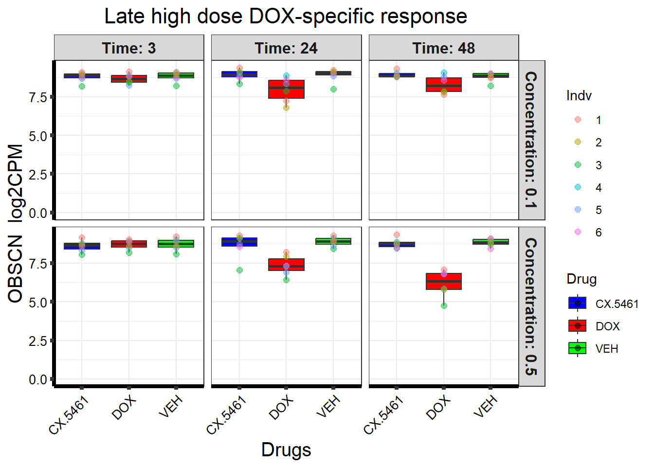
| Version | Author | Date |
|---|---|---|
| ebfddcd | sayanpaul01 | 2025-02-23 |
📌 Corr-motif set Abs logFC boxplots
📌 Read and Process DEG Data
# Load DEGs Data
CX_0.1_3 <- read.csv("data/DEGs/Toptable_CX_0.1_3.csv")
CX_0.1_24 <- read.csv("data/DEGs/Toptable_CX_0.1_24.csv")
CX_0.1_48 <- read.csv("data/DEGs/Toptable_CX_0.1_48.csv")
CX_0.5_3 <- read.csv("data/DEGs/Toptable_CX_0.5_3.csv")
CX_0.5_24 <- read.csv("data/DEGs/Toptable_CX_0.5_24.csv")
CX_0.5_48 <- read.csv("data/DEGs/Toptable_CX_0.5_48.csv")

DOX_0.1_3 <- read.csv("data/DEGs/Toptable_DOX_0.1_3.csv")
DOX_0.1_24 <- read.csv("data/DEGs/Toptable_DOX_0.1_24.csv")
DOX_0.1_48 <- read.csv("data/DEGs/Toptable_DOX_0.1_48.csv")
DOX_0.5_3 <- read.csv("data/DEGs/Toptable_DOX_0.5_3.csv")
DOX_0.5_24 <- read.csv("data/DEGs/Toptable_DOX_0.5_24.csv")
DOX_0.5_48 <- read.csv("data/DEGs/Toptable_DOX_0.5_48.csv")

Toptable_CX_0.1_3_df<- data.frame(CX_0.1_3)
Toptable_CX_0.1_24_df<- data.frame(CX_0.1_24)
Toptable_CX_0.1_48_df<- data.frame(CX_0.1_48)
Toptable_CX_0.5_3_df<- data.frame(CX_0.5_3)
Toptable_CX_0.5_24_df<- data.frame(CX_0.5_24)
Toptable_CX_0.5_48_df<- data.frame(CX_0.5_48)
Toptable_DOX_0.1_3_df<- data.frame(DOX_0.1_3)
Toptable_DOX_0.1_24_df<- data.frame(DOX_0.1_24)
Toptable_DOX_0.1_48_df<- data.frame(DOX_0.1_48)
Toptable_DOX_0.5_3_df<- data.frame(DOX_0.5_3)
Toptable_DOX_0.5_24_df<- data.frame(DOX_0.5_24)
Toptable_DOX_0.5_48_df<- data.frame(DOX_0.5_48)
📌 Non response abs logFC boxplots
# Extract Entrez_IDs from set1
non_response_entrez_ids <- prob_all_1

all_toptables <- bind_rows(
  Toptable_CX_0.1_3_df %>% mutate(Drug = "CX.5461", Concentration = 0.1, Timepoint = "3"),
  Toptable_CX_0.1_24_df %>% mutate(Drug = "CX.5461", Concentration = 0.1, Timepoint = "24"),
  Toptable_CX_0.1_48_df %>% mutate(Drug = "CX.5461", Concentration = 0.1, Timepoint = "48"),
  Toptable_CX_0.5_3_df %>% mutate(Drug = "CX.5461", Concentration = 0.5, Timepoint = "3"),
  Toptable_CX_0.5_24_df %>% mutate(Drug = "CX.5461", Concentration = 0.5, Timepoint = "24"),
  Toptable_CX_0.5_48_df %>% mutate(Drug = "CX.5461", Concentration = 0.5, Timepoint = "48"),
  Toptable_DOX_0.1_3_df %>% mutate(Drug = "DOX", Concentration = 0.1, Timepoint = "3"),
  Toptable_DOX_0.1_24_df %>% mutate(Drug = "DOX", Concentration = 0.1, Timepoint = "24"),
  Toptable_DOX_0.1_48_df %>% mutate(Drug = "DOX", Concentration = 0.1, Timepoint = "48"),
  Toptable_DOX_0.5_3_df %>% mutate(Drug = "DOX", Concentration = 0.5, Timepoint = "3"),
  Toptable_DOX_0.5_24_df %>% mutate(Drug = "DOX", Concentration = 0.5, Timepoint = "24"),
  Toptable_DOX_0.5_48_df %>% mutate(Drug = "DOX", Concentration = 0.5, Timepoint = "48")
)

# Filter and visualize data for shared late response genes
filtered_toptables <- all_toptables %>%
  filter(Entrez_ID %in% non_response_entrez_ids)

# Filter and visualize data with exact same font size and bold styling for concentration and timepoints
filtered_toptables %>%
  mutate(absFC = abs(logFC)) %>%  # Compute absolute log fold change
  mutate(
    Drug = factor(Drug, levels = c("CX.5461", "DOX")),  # Factorize Drug with CX.5461 first
    Timepoint = factor(Timepoint, levels = c("3", "24", "48"), labels = c("Timepoint: 3 hours", "Timepoint: 24 hours", "Timepoint: 48 hours")),
    Concentration = factor(Concentration, levels = c(0.1, 0.5), labels = c("Concentration: 0.1", "Concentration: 0.5"))
  ) %>%
  ggplot(aes(x = Drug, y = absFC)) +
  geom_boxplot(aes(fill = Drug)) +
  scale_fill_manual(values = c("CX.5461" = "blue", "DOX" = "red")) +  # Updated color palette
  guides(fill = guide_legend(title = "Treatment")) +
  facet_grid(Concentration ~ Timepoint) +  # Facet by Concentration and Timepoint
  theme_bw() +
  xlab("Drugs") +
  ylab("|Log Fold Change|") +
  ggtitle("|Log Fold| for Non-Response Genes") +
  theme(
    plot.title = element_text(size = rel(1.5), hjust = 0.5),
    axis.title = element_text(size = 15, color = "black"),
    axis.line = element_line(linewidth = 1.5),
    strip.background = element_rect(fill = "gray"),  # Set strip background to gray
    strip.text = element_text(size = 12, color = "black", face = "bold"),  # Unified styling for all facet labels
    axis.text.x = element_text(size = 8, color = "black", angle = 15)
  )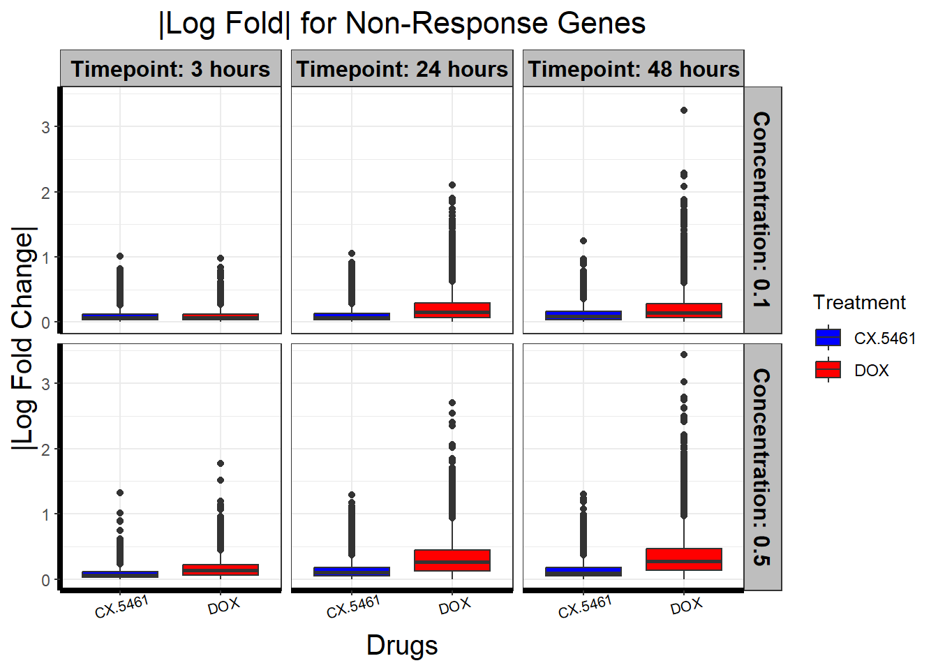
| Version | Author | Date |
|---|---|---|
| 2862c42 | sayanpaul01 | 2025-02-24 |
📌 CX_DOX shared late response abs logFC boxplots
# Extract Entrez_IDs from set2
shared_late_response_entrez_ids <- prob_all_2

# Combine all subset_toptables into a single data frame with additional metadata columns
all_toptables <- bind_rows(
  Toptable_CX_0.1_3_df %>% mutate(Drug = "CX.5461", Concentration = 0.1, Timepoint = "3"),
  Toptable_CX_0.1_24_df %>% mutate(Drug = "CX.5461", Concentration = 0.1, Timepoint = "24"),
  Toptable_CX_0.1_48_df %>% mutate(Drug = "CX.5461", Concentration = 0.1, Timepoint = "48"),
  Toptable_CX_0.5_3_df %>% mutate(Drug = "CX.5461", Concentration = 0.5, Timepoint = "3"),
  Toptable_CX_0.5_24_df %>% mutate(Drug = "CX.5461", Concentration = 0.5, Timepoint = "24"),
  Toptable_CX_0.5_48_df %>% mutate(Drug = "CX.5461", Concentration = 0.5, Timepoint = "48"),
  Toptable_DOX_0.1_3_df %>% mutate(Drug = "DOX", Concentration = 0.1, Timepoint = "3"),
  Toptable_DOX_0.1_24_df %>% mutate(Drug = "DOX", Concentration = 0.1, Timepoint = "24"),
  Toptable_DOX_0.1_48_df %>% mutate(Drug = "DOX", Concentration = 0.1, Timepoint = "48"),
  Toptable_DOX_0.5_3_df %>% mutate(Drug = "DOX", Concentration = 0.5, Timepoint = "3"),
  Toptable_DOX_0.5_24_df %>% mutate(Drug = "DOX", Concentration = 0.5, Timepoint = "24"),
  Toptable_DOX_0.5_48_df %>% mutate(Drug = "DOX", Concentration = 0.5, Timepoint = "48")
)

# Filter and visualize data for shared late response genes
filtered_toptables <- all_toptables %>%
  filter(Entrez_ID %in% shared_late_response_entrez_ids)

filtered_toptables %>%
  mutate(absFC = abs(logFC)) %>%  # Compute absolute log fold change
  mutate(
    Drug = factor(Drug, levels = c("CX.5461", "DOX")),  # Factorize Drug with CX.5461 first
    Timepoint = factor(Timepoint, levels = c("3", "24", "48"), labels = c("Timepoint: 3 hours", "Timepoint: 24 hours", "Timepoint: 48 hours")),
    Concentration = factor(Concentration, levels = c(0.1, 0.5), labels = c("Concentration: 0.1", "Concentration: 0.5"))
  ) %>%
  ggplot(aes(x = Drug, y = absFC)) +
  geom_boxplot(aes(fill = Drug)) +
  scale_fill_manual(values = c("CX.5461" = "blue", "DOX" = "red")) +  # Updated color palette
  guides(fill = guide_legend(title = "Treatment")) +
  facet_grid(Concentration ~ Timepoint) +  # Facet by Concentration and Timepoint
  theme_bw() +
  xlab("Drugs") +
  ylab("|Log Fold Change|") +
  ggtitle("|Log Fold| for CX_DOX shared late response Genes") +
  theme(
    plot.title = element_text(size = rel(1.5), hjust = 0.5),
    axis.title = element_text(size = 15, color = "black"),
    axis.line = element_line(linewidth = 1.5),
    strip.background = element_rect(fill = "gray"),  # Set strip background to gray
    strip.text = element_text(size = 12, color = "black", face = "bold"),  # Unified styling for all facet labels
    axis.text.x = element_text(size = 8, color = "black", angle = 15)
  )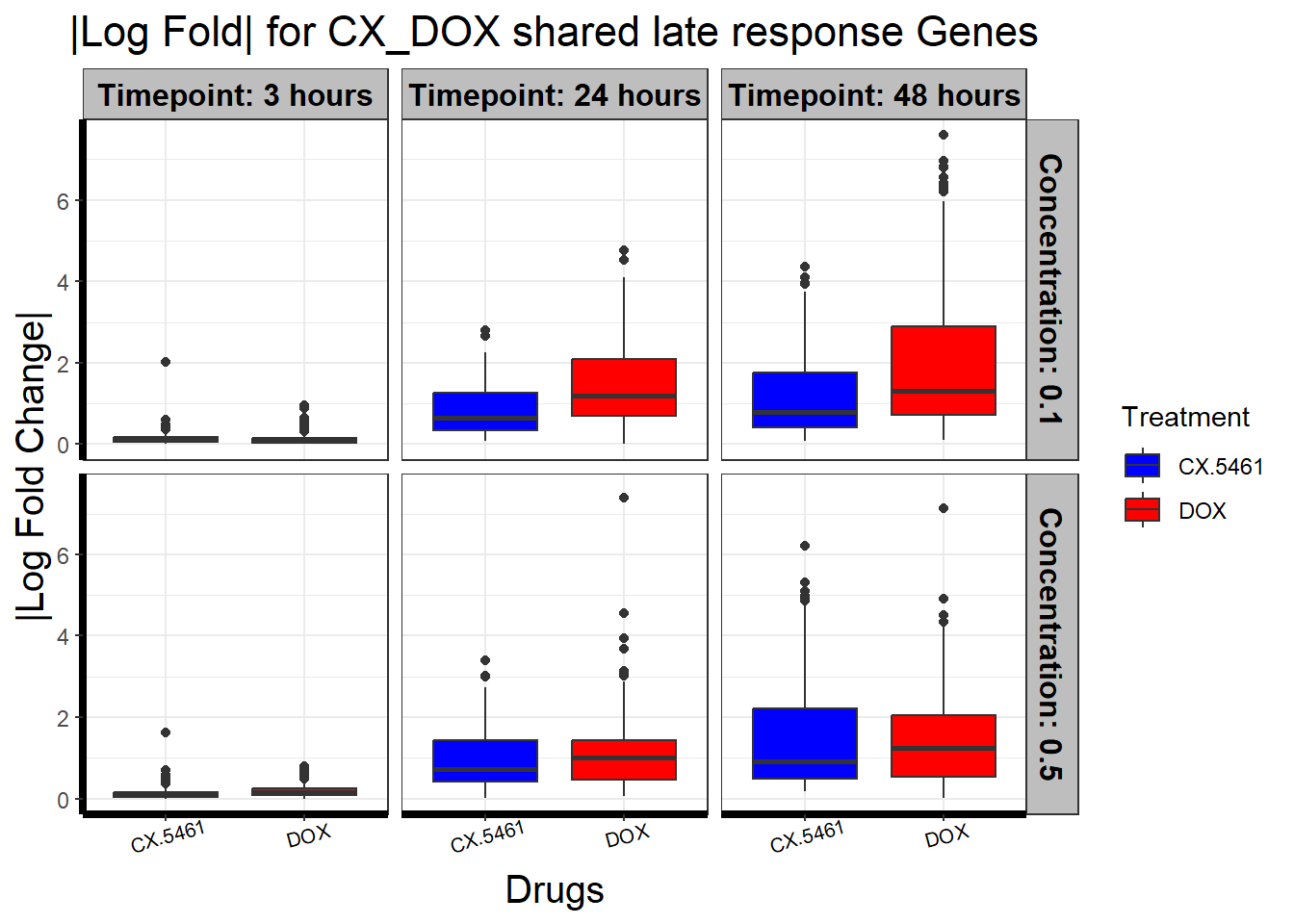
| Version | Author | Date |
|---|---|---|
| 2862c42 | sayanpaul01 | 2025-02-24 |
📌 DOX Specific response abs logFC boxplots
# Extract Entrez_IDs from set3
dox_specific_response_entrez_ids <- prob_all_3

# Combine all subset_toptables into a single data frame with additional metadata columns
all_toptables <- bind_rows(
  Toptable_CX_0.1_3_df %>% mutate(Drug = "CX.5461", Concentration = 0.1, Timepoint = "3"),
  Toptable_CX_0.1_24_df %>% mutate(Drug = "CX.5461", Concentration = 0.1, Timepoint = "24"),
  Toptable_CX_0.1_48_df %>% mutate(Drug = "CX.5461", Concentration = 0.1, Timepoint = "48"),
  Toptable_CX_0.5_3_df %>% mutate(Drug = "CX.5461", Concentration = 0.5, Timepoint = "3"),
  Toptable_CX_0.5_24_df %>% mutate(Drug = "CX.5461", Concentration = 0.5, Timepoint = "24"),
  Toptable_CX_0.5_48_df %>% mutate(Drug = "CX.5461", Concentration = 0.5, Timepoint = "48"),
  Toptable_DOX_0.1_3_df %>% mutate(Drug = "DOX", Concentration = 0.1, Timepoint = "3"),
  Toptable_DOX_0.1_24_df %>% mutate(Drug = "DOX", Concentration = 0.1, Timepoint = "24"),
  Toptable_DOX_0.1_48_df %>% mutate(Drug = "DOX", Concentration = 0.1, Timepoint = "48"),
  Toptable_DOX_0.5_3_df %>% mutate(Drug = "DOX", Concentration = 0.5, Timepoint = "3"),
  Toptable_DOX_0.5_24_df %>% mutate(Drug = "DOX", Concentration = 0.5, Timepoint = "24"),
  Toptable_DOX_0.5_48_df %>% mutate(Drug = "DOX", Concentration = 0.5, Timepoint = "48")
)

# Filter and visualize data for DOX-specific response genes
filtered_toptables <- all_toptables %>%
  filter(Entrez_ID %in% dox_specific_response_entrez_ids)

filtered_toptables %>%
  mutate(absFC = abs(logFC)) %>%  # Compute absolute log fold change
  mutate(
    Drug = factor(Drug, levels = c("CX.5461", "DOX")),  # Factorize Drug with CX.5461 first
    Timepoint = factor(Timepoint, levels = c("3", "24", "48"), labels = c("Timepoint: 3 hours", "Timepoint: 24 hours", "Timepoint: 48 hours")),
    Concentration = factor(Concentration, levels = c(0.1, 0.5), labels = c("Concentration: 0.1", "Concentration: 0.5"))
  ) %>%
  ggplot(aes(x = Drug, y = absFC)) +
  geom_boxplot(aes(fill = Drug)) +
  scale_fill_manual(values = c("CX.5461" = "blue", "DOX" = "red")) +  # Updated color palette
  guides(fill = guide_legend(title = "Treatment")) +
  facet_grid(Concentration ~ Timepoint) +  # Facet by Concentration and Timepoint
  theme_bw() +
  xlab("Drugs") +
  ylab("|Log Fold Change|") +
  ggtitle("|Log Fold| for DOX-Specific Response Genes") +
  theme(
    plot.title = element_text(size = rel(1.5), hjust = 0.5),
    axis.title = element_text(size = 15, color = "black"),
    axis.line = element_line(linewidth = 1.5),
    strip.background = element_rect(fill = "gray"),  # Set strip background to gray
    strip.text = element_text(size = 12, color = "black", face = "bold"),  # Unified styling for all facet labels
    axis.text.x = element_text(size = 8, color = "black", angle = 15)
  )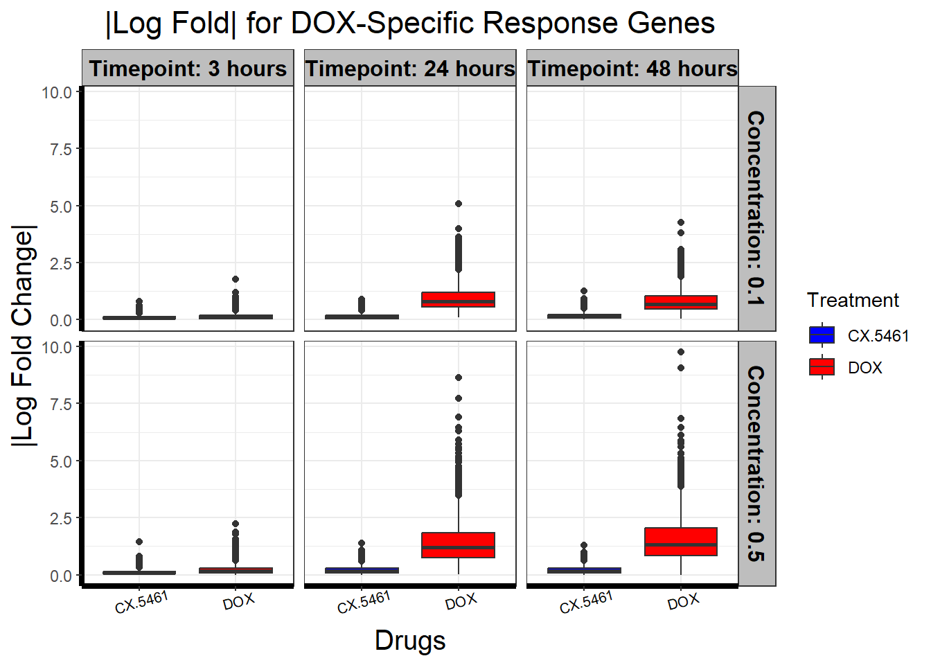
| Version | Author | Date |
|---|---|---|
| 2862c42 | sayanpaul01 | 2025-02-24 |
📌 Late high dose DOX-specific response abs logFC boxplots
# Extract Entrez_IDs from set4
late_high_dose_dox_entrez_ids <- prob_all_4

# Combine all subset_toptables into a single data frame with additional metadata columns
all_toptables <- bind_rows(
  Toptable_CX_0.1_3_df %>% mutate(Drug = "CX.5461", Concentration = 0.1, Timepoint = "3"),
  Toptable_CX_0.1_24_df %>% mutate(Drug = "CX.5461", Concentration = 0.1, Timepoint = "24"),
  Toptable_CX_0.1_48_df %>% mutate(Drug = "CX.5461", Concentration = 0.1, Timepoint = "48"),
  Toptable_CX_0.5_3_df %>% mutate(Drug = "CX.5461", Concentration = 0.5, Timepoint = "3"),
  Toptable_CX_0.5_24_df %>% mutate(Drug = "CX.5461", Concentration = 0.5, Timepoint = "24"),
  Toptable_CX_0.5_48_df %>% mutate(Drug = "CX.5461", Concentration = 0.5, Timepoint = "48"),
  Toptable_DOX_0.1_3_df %>% mutate(Drug = "DOX", Concentration = 0.1, Timepoint = "3"),
  Toptable_DOX_0.1_24_df %>% mutate(Drug = "DOX", Concentration = 0.1, Timepoint = "24"),
  Toptable_DOX_0.1_48_df %>% mutate(Drug = "DOX", Concentration = 0.1, Timepoint = "48"),
  Toptable_DOX_0.5_3_df %>% mutate(Drug = "DOX", Concentration = 0.5, Timepoint = "3"),
  Toptable_DOX_0.5_24_df %>% mutate(Drug = "DOX", Concentration = 0.5, Timepoint = "24"),
  Toptable_DOX_0.5_48_df %>% mutate(Drug = "DOX", Concentration = 0.5, Timepoint = "48")
)

# Filter and visualize data for late high dose DOX-specific response genes
filtered_toptables <- all_toptables %>%
  filter(Entrez_ID %in% late_high_dose_dox_entrez_ids)

filtered_toptables %>%
  mutate(absFC = abs(logFC)) %>%  # Compute absolute log fold change
  mutate(
    Drug = factor(Drug, levels = c("CX.5461", "DOX")),  # Factorize Drug with CX.5461 first
    Timepoint = factor(Timepoint, levels = c("3", "24", "48"), labels = c("Timepoint: 3 hours", "Timepoint: 24 hours", "Timepoint: 48 hours")),
    Concentration = factor(Concentration, levels = c(0.1, 0.5), labels = c("Concentration: 0.1", "Concentration: 0.5"))
  ) %>%
  ggplot(aes(x = Drug, y = absFC)) +
  geom_boxplot(aes(fill = Drug)) +
  scale_fill_manual(values = c("CX.5461" = "blue", "DOX" = "red")) +  # Updated color palette
  guides(fill = guide_legend(title = "Treatment")) +
  facet_grid(Concentration ~ Timepoint) +  # Facet by Concentration and Timepoint
  theme_bw() +
  xlab("Drugs") +
  ylab("|Log Fold Change|") +
  ggtitle("|Log Fold| for Late High Dose DOX-Specific Response Genes") +
  theme(
    plot.title = element_text(size = rel(1.5), hjust = 0.5),
    axis.title = element_text(size = 15, color = "black"),
    axis.line = element_line(linewidth = 1.5),
    strip.background = element_rect(fill = "gray"),  # Set strip background to gray
    strip.text = element_text(size = 12, color = "black", face = "bold"),  # Unified styling for all facet labels
    axis.text.x = element_text(size = 8, color = "black", angle = 15)
  )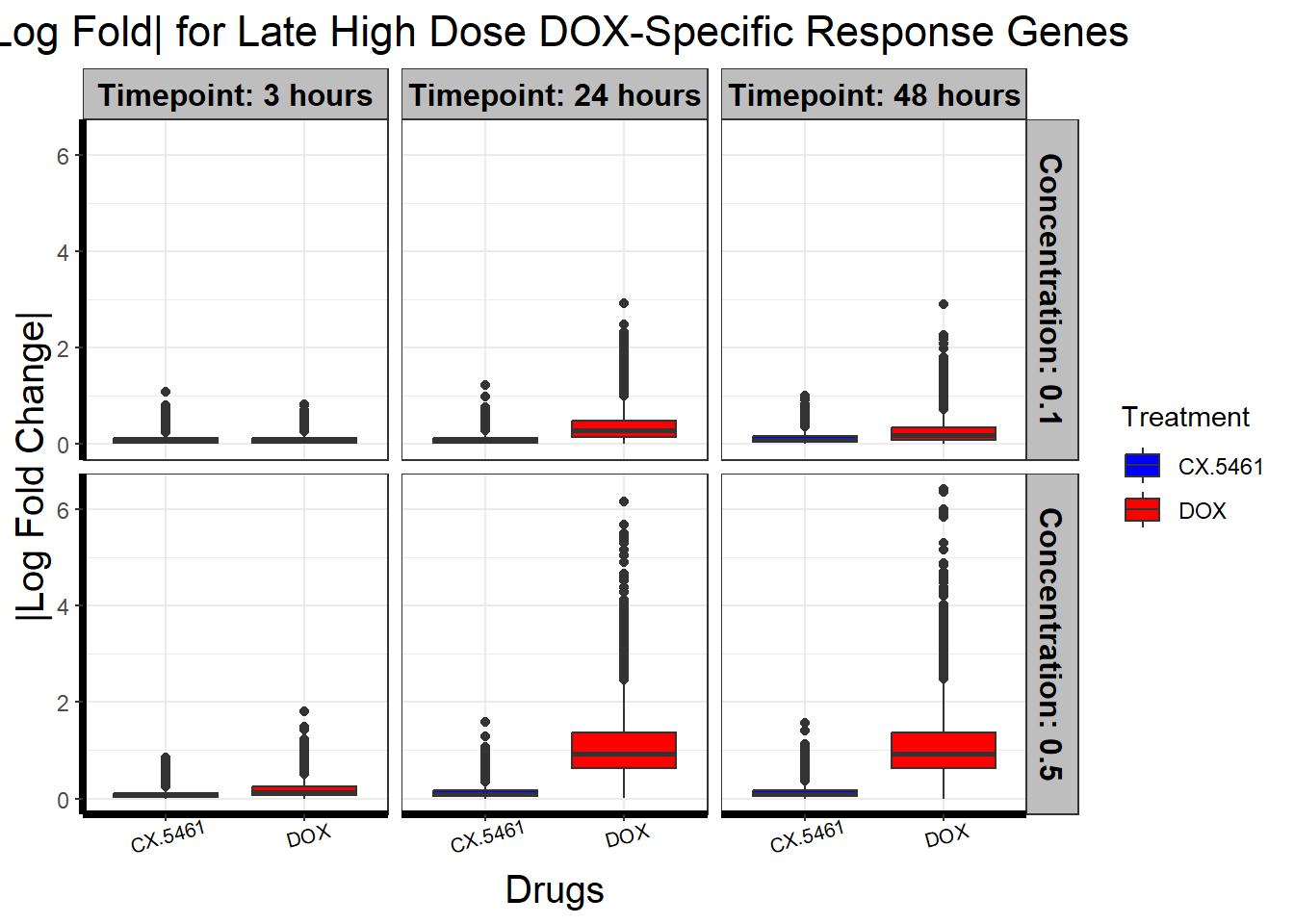
| Version | Author | Date |
|---|---|---|
| 2862c42 | sayanpaul01 | 2025-02-24 |
📌 Corr-motif set mean (Abs logFC) across timepoints
all_toptables <- bind_rows(
  Toptable_CX_0.1_3_df %>% mutate(Drug = "CX.5461", Concentration = 0.1, Timepoint = "3"),
  Toptable_CX_0.1_24_df %>% mutate(Drug = "CX.5461", Concentration = 0.1, Timepoint = "24"),
  Toptable_CX_0.1_48_df %>% mutate(Drug = "CX.5461", Concentration = 0.1, Timepoint = "48"),
  Toptable_CX_0.5_3_df %>% mutate(Drug = "CX.5461", Concentration = 0.5, Timepoint = "3"),
  Toptable_CX_0.5_24_df %>% mutate(Drug = "CX.5461", Concentration = 0.5, Timepoint = "24"),
  Toptable_CX_0.5_48_df %>% mutate(Drug = "CX.5461", Concentration = 0.5, Timepoint = "48"),
  Toptable_DOX_0.1_3_df %>% mutate(Drug = "DOX", Concentration = 0.1, Timepoint = "3"),
  Toptable_DOX_0.1_24_df %>% mutate(Drug = "DOX", Concentration = 0.1, Timepoint = "24"),
  Toptable_DOX_0.1_48_df %>% mutate(Drug = "DOX", Concentration = 0.1, Timepoint = "48"),
  Toptable_DOX_0.5_3_df %>% mutate(Drug = "DOX", Concentration = 0.5, Timepoint = "3"),
  Toptable_DOX_0.5_24_df %>% mutate(Drug = "DOX", Concentration = 0.5, Timepoint = "24"),
  Toptable_DOX_0.5_48_df %>% mutate(Drug = "DOX", Concentration = 0.5, Timepoint = "48")
)

# Convert Entrez_ID in `all_toptables` to character for proper matching
all_toptables <- all_toptables %>% mutate(Entrez_ID = as.character(Entrez_ID))

# Define datasets for filtering (lists of Entrez IDs)
data_sets <- list(
  "Non Response" = prob_all_1,
  "CX_DOX Shared\nLate Response" = prob_all_2,
  "DOX-Specific Response" = prob_all_3,
  "Late High Dose\nDOX-Specific Response" = prob_all_4
)

# Filter datasets and add labels
data_combined <- bind_rows(lapply(names(data_sets), function(label) {
  all_toptables %>%
    filter(Entrez_ID %in% data_sets[[label]]) %>%  # Use list directly for filtering
    mutate(Dataset = label)
}))

# Ensure `logFC` column exists before computing mean absolute logFC
if (!"logFC" %in% colnames(data_combined)) {
  stop("Column `logFC` is missing in `data_combined`. Ensure that `all_toptables` has `logFC`.")
}

# Compute mean absolute logFC grouped by Dataset, Drug, Concentration, and Timepoint
data_summary <- data_combined %>%
  mutate(abs_logFC = abs(logFC)) %>%  # Take absolute log fold change
  group_by(Dataset, Drug, Concentration, Timepoint) %>%
  dplyr::summarize(mean_abs_logFC = mean(abs_logFC, na.rm = TRUE), .groups = "drop") %>%
  as.data.frame()

# Convert factors for plotting
data_summary <- data_summary %>%
  mutate(
    Timepoint = factor(Timepoint, levels = c("3", "24", "48"), labels = c("3 hours", "24 hours", "48 hours")),
    Concentration = factor(Concentration, levels = c(0.1, 0.5)),
    Dataset = factor(Dataset, levels = c("Non Response", "CX_DOX Shared\nLate Response", "DOX-Specific Response", "Late High Dose\nDOX-Specific Response"))
  )

# Define custom drug palette
drug_palette <- c("CX.5461" = "blue", "DOX" = "red")

# Plot the data for absolute logFC
ggplot(data_summary, aes(x = Timepoint, y = mean_abs_logFC, group = Drug, color = Drug)) +
  geom_point(size = 3) +
  geom_line(size = 1.2) +
  scale_color_manual(values = drug_palette) +
  ylim(0, 2) +  # Adjust the Y-axis for better visualization
  facet_grid(Dataset ~ Concentration) +
  theme_bw() +
  labs(
    x = "Timepoints",
    y = "Mean |Log Fold Change|",
    title = "Average |Log Fold Change| Across Motifs and Concentrations",
    color = "Drug"
  ) +
  theme(
    plot.title = element_text(size = rel(1.5), hjust = 0.5),
    axis.title = element_text(size = 15, color = "black"),
    axis.text = element_text(size = 12, color = "black"),
    strip.text = element_text(size = 12, color = "black", face = "bold"),
    legend.title = element_text(size = 14),
    legend.text = element_text(size = 12)
  )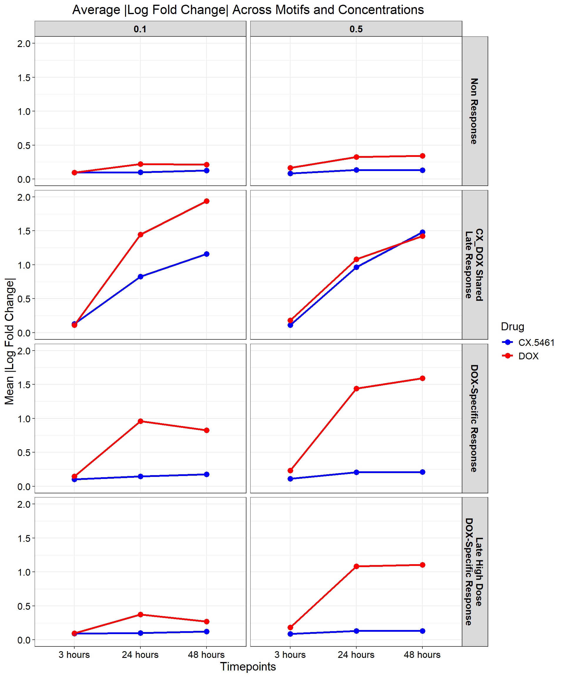
| Version | Author | Date |
|---|---|---|
| 2862c42 | sayanpaul01 | 2025-02-24 |
📌 Corr-motif set logFC boxplots
📌 Non response logFC boxplots
# Extract Entrez_IDs from set1
non_response_entrez_ids <- prob_all_1

# Combine all subset_toptables into a single data frame with additional metadata columns
all_toptables <- bind_rows(
  Toptable_CX_0.1_3_df %>% mutate(Drug = "CX.5461", Concentration = 0.1, Timepoint = "3"),
  Toptable_CX_0.1_24_df %>% mutate(Drug = "CX.5461", Concentration = 0.1, Timepoint = "24"),
  Toptable_CX_0.1_48_df %>% mutate(Drug = "CX.5461", Concentration = 0.1, Timepoint = "48"),
  Toptable_CX_0.5_3_df %>% mutate(Drug = "CX.5461", Concentration = 0.5, Timepoint = "3"),
  Toptable_CX_0.5_24_df %>% mutate(Drug = "CX.5461", Concentration = 0.5, Timepoint = "24"),
  Toptable_CX_0.5_48_df %>% mutate(Drug = "CX.5461", Concentration = 0.5, Timepoint = "48"),
  Toptable_DOX_0.1_3_df %>% mutate(Drug = "DOX", Concentration = 0.1, Timepoint = "3"),
  Toptable_DOX_0.1_24_df %>% mutate(Drug = "DOX", Concentration = 0.1, Timepoint = "24"),
  Toptable_DOX_0.1_48_df %>% mutate(Drug = "DOX", Concentration = 0.1, Timepoint = "48"),
  Toptable_DOX_0.5_3_df %>% mutate(Drug = "DOX", Concentration = 0.5, Timepoint = "3"),
  Toptable_DOX_0.5_24_df %>% mutate(Drug = "DOX", Concentration = 0.5, Timepoint = "24"),
  Toptable_DOX_0.5_48_df %>% mutate(Drug = "DOX", Concentration = 0.5, Timepoint = "48")
)


# Filter and visualize data for shared late response genes
filtered_toptables <- all_toptables %>%
  filter(Entrez_ID %in% non_response_entrez_ids)

# Visualization of logFC for non-response genes
filtered_toptables %>%
  mutate(
    Drug = factor(Drug, levels = c("CX.5461", "DOX")),  # Factorize Drug with CX.5461 first
    Timepoint = factor(Timepoint, levels = c("3", "24", "48"), labels = c("Timepoint: 3 hours", "Timepoint: 24 hours", "Timepoint: 48 hours")),
    Concentration = factor(Concentration, levels = c(0.1, 0.5), labels = c("Concentration: 0.1", "Concentration: 0.5"))
  ) %>%
  ggplot(aes(x = Drug, y = logFC)) +  # Plot logFC directly
  geom_boxplot(aes(fill = Drug)) +
  scale_fill_manual(values = c("CX.5461" = "blue", "DOX" = "red")) +  # Updated color palette
  guides(fill = guide_legend(title = "Treatment")) +
  facet_grid(Concentration ~ Timepoint) +  # Facet by Concentration and Timepoint
  theme_bw() +
  xlab("Drugs") +
  ylab("Log Fold Change") +  # Updated y-axis label
  ggtitle("Log Fold Change for Non-Response Genes") +
  theme(
    plot.title = element_text(size = rel(1.5), hjust = 0.5),
    axis.title = element_text(size = 15, color = "black"),
    axis.line = element_line(linewidth = 1.5),
    strip.background = element_rect(fill = "gray"),  # Set strip background to gray
    strip.text = element_text(size = 12, color = "black", face = "bold"),  # Unified styling for all facet labels
    axis.text.x = element_text(size = 8, color = "black", angle = 15)
  )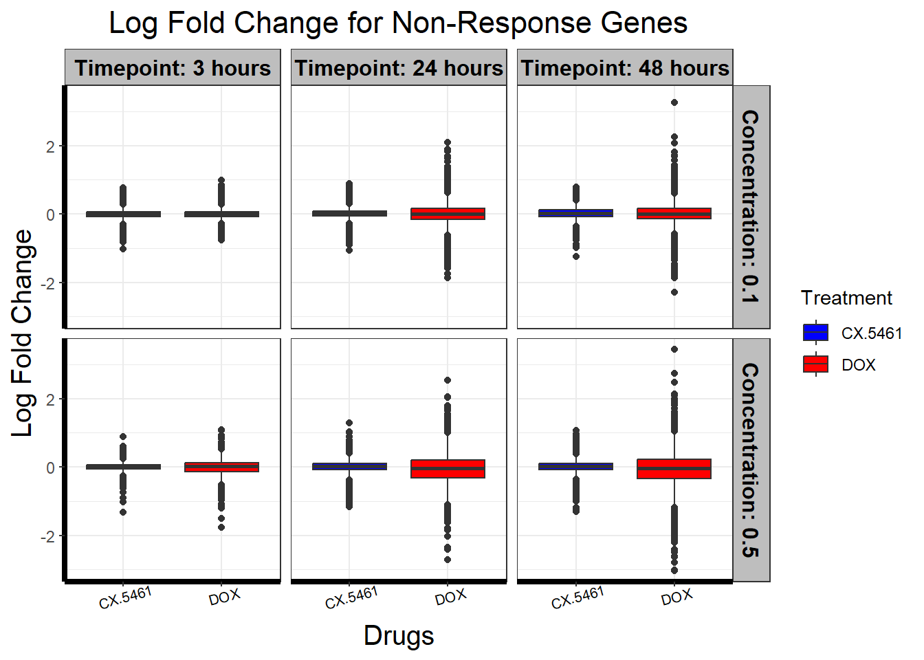
| Version | Author | Date |
|---|---|---|
| 2862c42 | sayanpaul01 | 2025-02-24 |
📌 CX_DOX Shared Late Response logFC boxplots
# Extract Entrez_IDs from set2
cx_dox_shared_entrez_ids <- prob_all_2

# Combine all subset_toptables into a single data frame with additional metadata columns
all_toptables <- bind_rows(
  Toptable_CX_0.1_3_df %>% mutate(Drug = "CX.5461", Concentration = 0.1, Timepoint = "3"),
  Toptable_CX_0.1_24_df %>% mutate(Drug = "CX.5461", Concentration = 0.1, Timepoint = "24"),
  Toptable_CX_0.1_48_df %>% mutate(Drug = "CX.5461", Concentration = 0.1, Timepoint = "48"),
  Toptable_CX_0.5_3_df %>% mutate(Drug = "CX.5461", Concentration = 0.5, Timepoint = "3"),
  Toptable_CX_0.5_24_df %>% mutate(Drug = "CX.5461", Concentration = 0.5, Timepoint = "24"),
  Toptable_CX_0.5_48_df %>% mutate(Drug = "CX.5461", Concentration = 0.5, Timepoint = "48"),
  Toptable_DOX_0.1_3_df %>% mutate(Drug = "DOX", Concentration = 0.1, Timepoint = "3"),
  Toptable_DOX_0.1_24_df %>% mutate(Drug = "DOX", Concentration = 0.1, Timepoint = "24"),
  Toptable_DOX_0.1_48_df %>% mutate(Drug = "DOX", Concentration = 0.1, Timepoint = "48"),
  Toptable_DOX_0.5_3_df %>% mutate(Drug = "DOX", Concentration = 0.5, Timepoint = "3"),
  Toptable_DOX_0.5_24_df %>% mutate(Drug = "DOX", Concentration = 0.5, Timepoint = "24"),
  Toptable_DOX_0.5_48_df %>% mutate(Drug = "DOX", Concentration = 0.5, Timepoint = "48")
)

# Filter and visualize data for CX_DOX shared late response genes
filtered_toptables <- all_toptables %>%
  filter(Entrez_ID %in% cx_dox_shared_entrez_ids)

# Visualization of logFC for CX_DOX shared late response genes
filtered_toptables %>%
  mutate(
    Drug = factor(Drug, levels = c("CX.5461", "DOX")),  # Factorize Drug with CX.5461 first
    Timepoint = factor(Timepoint, levels = c("3", "24", "48"), labels = c("Timepoint: 3 hours", "Timepoint: 24 hours", "Timepoint: 48 hours")),
    Concentration = factor(Concentration, levels = c(0.1, 0.5), labels = c("Concentration: 0.1", "Concentration: 0.5"))
  ) %>%
  ggplot(aes(x = Drug, y = logFC)) +  # Plot logFC directly
  geom_boxplot(aes(fill = Drug)) +
  scale_fill_manual(values = c("CX.5461" = "blue", "DOX" = "red")) +  # Updated color palette
  guides(fill = guide_legend(title = "Treatment")) +
  facet_grid(Concentration ~ Timepoint) +  # Facet by Concentration and Timepoint
  theme_bw() +
  theme_bw() +
  xlab("Drugs") +
  ylab("Log Fold Change") +  # Updated y-axis label
  ggtitle("Log Fold Change for CX_DOX Shared Late Response Genes") +
  theme(
    plot.title = element_text(size = rel(1.5), hjust = 0.5),
    axis.title = element_text(size = 15, color = "black"),
    axis.line = element_line(linewidth = 1.5),
    strip.background = element_rect(fill = "gray"),  # Set strip background to gray
    strip.text = element_text(size = 12, color = "black", face = "bold"),  # Unified styling for all facet labels
    axis.text.x = element_text(size = 8, color = "black", angle = 15)
  )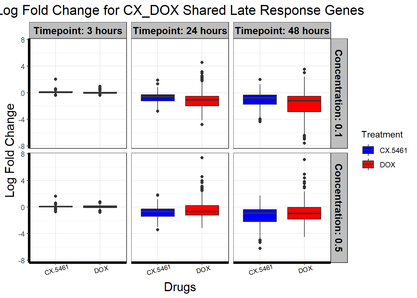
| Version | Author | Date |
|---|---|---|
| 2862c42 | sayanpaul01 | 2025-02-24 |
📌 DOX-Specific Response logFC boxplots
# Extract Entrez_IDs from set3
dox_specific_entrez_ids <- prob_all_3

# Combine all subset_toptables into a single data frame with additional metadata columns
all_toptables <- bind_rows(
  Toptable_CX_0.1_3_df %>% mutate(Drug = "CX.5461", Concentration = 0.1, Timepoint = "3"),
  Toptable_CX_0.1_24_df %>% mutate(Drug = "CX.5461", Concentration = 0.1, Timepoint = "24"),
  Toptable_CX_0.1_48_df %>% mutate(Drug = "CX.5461", Concentration = 0.1, Timepoint = "48"),
  Toptable_CX_0.5_3_df %>% mutate(Drug = "CX.5461", Concentration = 0.5, Timepoint = "3"),
  Toptable_CX_0.5_24_df %>% mutate(Drug = "CX.5461", Concentration = 0.5, Timepoint = "24"),
  Toptable_CX_0.5_48_df %>% mutate(Drug = "CX.5461", Concentration = 0.5, Timepoint = "48"),
  Toptable_DOX_0.1_3_df %>% mutate(Drug = "DOX", Concentration = 0.1, Timepoint = "3"),
  Toptable_DOX_0.1_24_df %>% mutate(Drug = "DOX", Concentration = 0.1, Timepoint = "24"),
  Toptable_DOX_0.1_48_df %>% mutate(Drug = "DOX", Concentration = 0.1, Timepoint = "48"),
  Toptable_DOX_0.5_3_df %>% mutate(Drug = "DOX", Concentration = 0.5, Timepoint = "3"),
  Toptable_DOX_0.5_24_df %>% mutate(Drug = "DOX", Concentration = 0.5, Timepoint = "24"),
  Toptable_DOX_0.5_48_df %>% mutate(Drug = "DOX", Concentration = 0.5, Timepoint = "48")
)

# Filter and visualize data for DOX-specific response genes
filtered_toptables <- all_toptables %>%
  filter(Entrez_ID %in% dox_specific_entrez_ids)

# Visualization of logFC for DOX-specific response genes
filtered_toptables %>%
  mutate(
    Drug = factor(Drug, levels = c("CX.5461", "DOX")),  # Factorize Drug with CX.5461 first
    Timepoint = factor(Timepoint, levels = c("3", "24", "48"), labels = c("Timepoint: 3 hours", "Timepoint: 24 hours", "Timepoint: 48 hours")),
    Concentration = factor(Concentration, levels = c(0.1, 0.5), labels = c("Concentration: 0.1", "Concentration: 0.5"))
  ) %>%
  ggplot(aes(x = Drug, y = logFC)) +  # Plot logFC directly
  geom_boxplot(aes(fill = Drug)) +
  scale_fill_manual(values = c("CX.5461" = "blue", "DOX" = "red")) +  # Updated color palette
  guides(fill = guide_legend(title = "Treatment")) +
  facet_grid(Concentration ~ Timepoint) +  # Facet by Concentration and Timepoint
  theme_bw() +
  xlab("Drugs") +
  ylab("Log Fold Change") +  # Updated y-axis label
  ggtitle("Log Fold Change for DOX-Specific Response Genes") +
  theme(
    plot.title = element_text(size = rel(1.5), hjust = 0.5),
    axis.title = element_text(size = 15, color = "black"),
    axis.line = element_line(linewidth = 1.5),
    strip.background = element_rect(fill = "gray"),  # Set strip background to gray
    strip.text = element_text(size = 12, color = "black", face = "bold"),  # Unified styling for all facet labels
    axis.text.x = element_text(size = 8, color = "black", angle = 15)
  )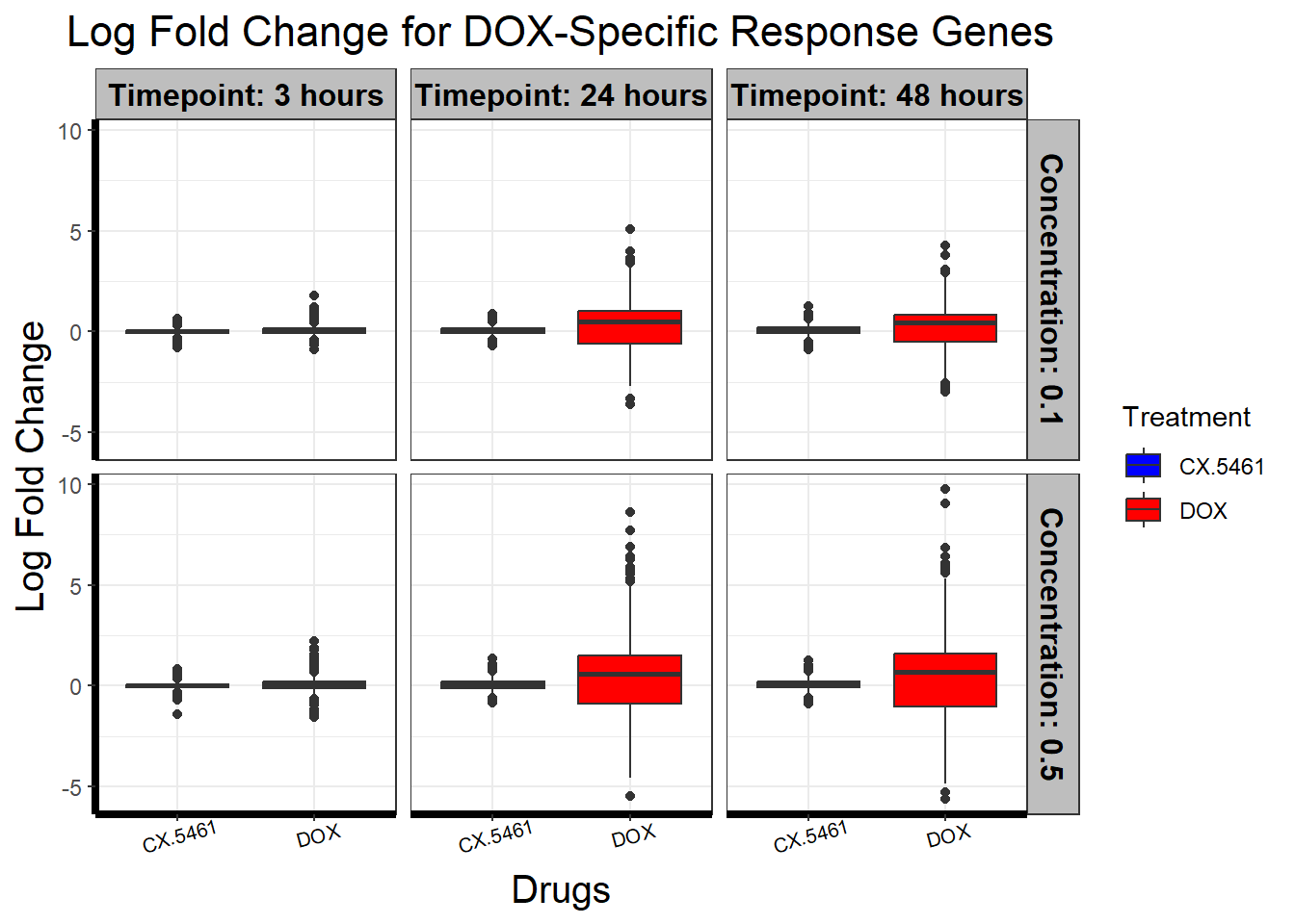
| Version | Author | Date |
|---|---|---|
| 2862c42 | sayanpaul01 | 2025-02-24 |
📌 Late High Dose DOX-Specific Response logFC boxplots
# Extract Entrez_IDs from set4
late_high_dose_dox_specific_entrez_ids <- prob_all_4

# Combine all subset_toptables into a single data frame with additional metadata columns
all_toptables <- bind_rows(
  Toptable_CX_0.1_3_df %>% mutate(Drug = "CX.5461", Concentration = 0.1, Timepoint = "3"),
  Toptable_CX_0.1_24_df %>% mutate(Drug = "CX.5461", Concentration = 0.1, Timepoint = "24"),
  Toptable_CX_0.1_48_df %>% mutate(Drug = "CX.5461", Concentration = 0.1, Timepoint = "48"),
  Toptable_CX_0.5_3_df %>% mutate(Drug = "CX.5461", Concentration = 0.5, Timepoint = "3"),
  Toptable_CX_0.5_24_df %>% mutate(Drug = "CX.5461", Concentration = 0.5, Timepoint = "24"),
  Toptable_CX_0.5_48_df %>% mutate(Drug = "CX.5461", Concentration = 0.5, Timepoint = "48"),
  Toptable_DOX_0.1_3_df %>% mutate(Drug = "DOX", Concentration = 0.1, Timepoint = "3"),
  Toptable_DOX_0.1_24_df %>% mutate(Drug = "DOX", Concentration = 0.1, Timepoint = "24"),
  Toptable_DOX_0.1_48_df %>% mutate(Drug = "DOX", Concentration = 0.1, Timepoint = "48"),
  Toptable_DOX_0.5_3_df %>% mutate(Drug = "DOX", Concentration = 0.5, Timepoint = "3"),
  Toptable_DOX_0.5_24_df %>% mutate(Drug = "DOX", Concentration = 0.5, Timepoint = "24"),
  Toptable_DOX_0.5_48_df %>% mutate(Drug = "DOX", Concentration = 0.5, Timepoint = "48")
)

# Filter and visualize data for Late High Dose DOX-Specific Response Genes
filtered_toptables <- all_toptables %>%
  filter(Entrez_ID %in% late_high_dose_dox_specific_entrez_ids)

# Visualization of logFC for Late High Dose DOX-Specific Response Genes
filtered_toptables %>%
  mutate(
    Drug = factor(Drug, levels = c("CX.5461", "DOX")),  # Factorize Drug with CX.5461 first
    Timepoint = factor(Timepoint, levels = c("3", "24", "48"), labels = c("Timepoint: 3 hours", "Timepoint: 24 hours", "Timepoint: 48 hours")),
    Concentration = factor(Concentration, levels = c(0.1, 0.5), labels = c("Concentration: 0.1", "Concentration: 0.5"))
  ) %>%
  ggplot(aes(x = Drug, y = logFC)) +  # Plot logFC directly
  geom_boxplot(aes(fill = Drug)) +
  scale_fill_manual(values = c("CX.5461" = "blue", "DOX" = "red")) +  # Updated color palette
  guides(fill = guide_legend(title = "Treatment")) +
  facet_grid(Concentration ~ Timepoint) +  # Facet by Concentration and Timepoint
  theme_bw() +
  xlab("Drugs") +
  ylab("Log Fold Change") +  # Updated y-axis label
  ggtitle("Log Fold Change for Late High Dose DOX-Specific Response Genes") +
  theme(
    plot.title = element_text(size = rel(1.5), hjust = 0.5),
    axis.title = element_text(size = 15, color = "black"),
    axis.line = element_line(linewidth = 1.5),
    strip.background = element_rect(fill = "gray"),  # Set strip background to gray
    strip.text = element_text(size = 12, color = "black", face = "bold"),  # Unified styling for all facet labels
    axis.text.x = element_text(size = 8, color = "black", angle = 15)
  )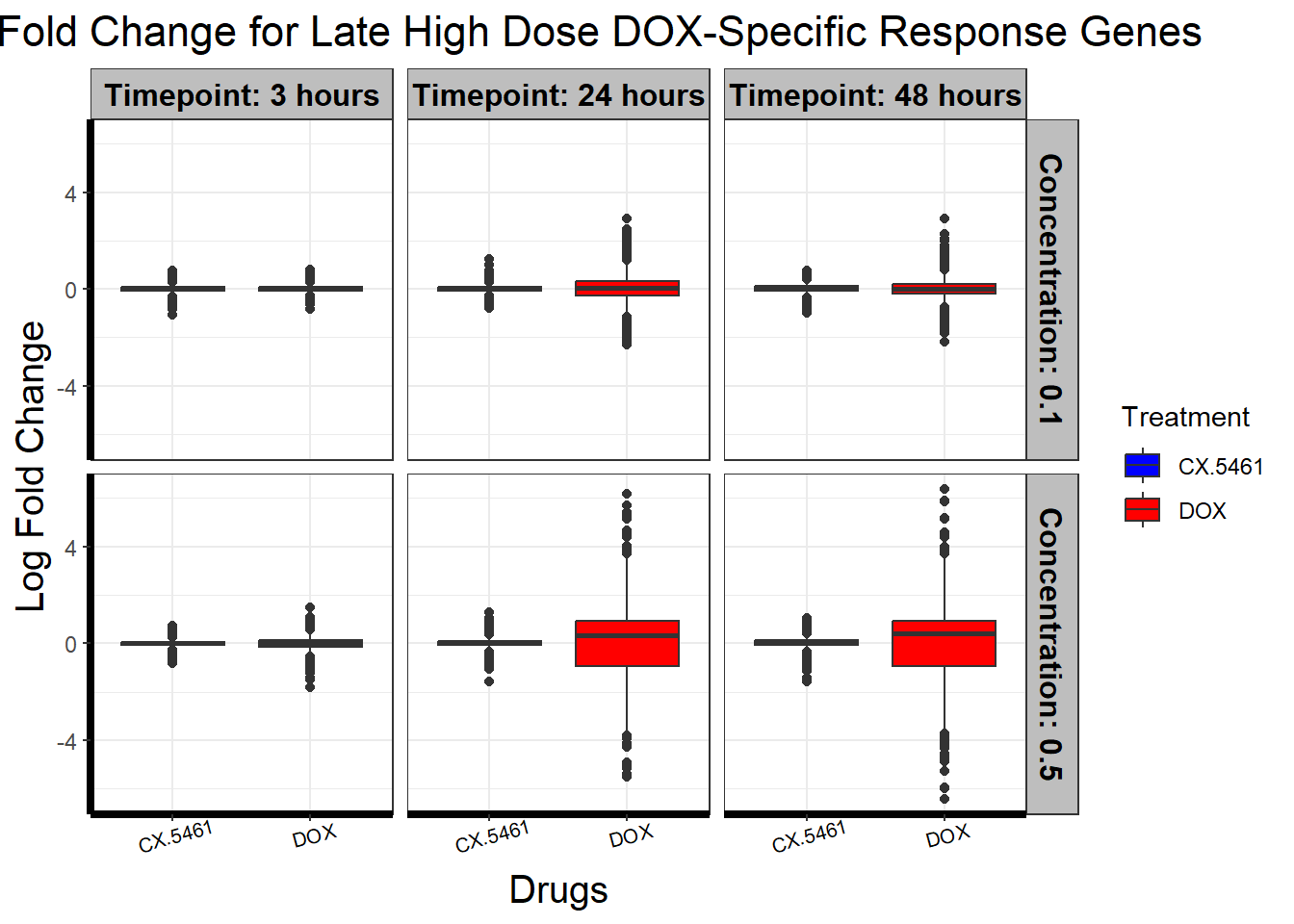
| Version | Author | Date |
|---|---|---|
| 2862c42 | sayanpaul01 | 2025-02-24 |
📌 Corr-motif set mean logFC across timepoints
# Combine all subset_toptables into a single data frame with additional metadata columns
all_toptables <- bind_rows(
  Toptable_CX_0.1_3_df %>% mutate(Drug = "CX.5461", Concentration = 0.1, Timepoint = "3"),
  Toptable_CX_0.1_24_df %>% mutate(Drug = "CX.5461", Concentration = 0.1, Timepoint = "24"),
  Toptable_CX_0.1_48_df %>% mutate(Drug = "CX.5461", Concentration = 0.1, Timepoint = "48"),
  Toptable_CX_0.5_3_df %>% mutate(Drug = "CX.5461", Concentration = 0.5, Timepoint = "3"),
  Toptable_CX_0.5_24_df %>% mutate(Drug = "CX.5461", Concentration = 0.5, Timepoint = "24"),
  Toptable_CX_0.5_48_df %>% mutate(Drug = "CX.5461", Concentration = 0.5, Timepoint = "48"),
  Toptable_DOX_0.1_3_df %>% mutate(Drug = "DOX", Concentration = 0.1, Timepoint = "3"),
  Toptable_DOX_0.1_24_df %>% mutate(Drug = "DOX", Concentration = 0.1, Timepoint = "24"),
  Toptable_DOX_0.1_48_df %>% mutate(Drug = "DOX", Concentration = 0.1, Timepoint = "48"),
  Toptable_DOX_0.5_3_df %>% mutate(Drug = "DOX", Concentration = 0.5, Timepoint = "3"),
  Toptable_DOX_0.5_24_df %>% mutate(Drug = "DOX", Concentration = 0.5, Timepoint = "24"),
  Toptable_DOX_0.5_48_df %>% mutate(Drug = "DOX", Concentration = 0.5, Timepoint = "48")
)

# Convert Entrez_ID in `all_toptables` to character for proper matching
all_toptables <- all_toptables %>% mutate(Entrez_ID = as.character(Entrez_ID))

# Define datasets for filtering (lists of Entrez IDs)
data_sets <- list(
  "Non Response" = prob_all_1,
  "CX_DOX Shared\nLate Response" = prob_all_2,
  "DOX-Specific Response" = prob_all_3,
  "Late High Dose\nDOX-Specific Response" = prob_all_4
)

# Filter datasets and add labels
data_combined <- bind_rows(lapply(names(data_sets), function(label) {
  all_toptables %>%
    filter(Entrez_ID %in% data_sets[[label]]) %>%  # Use list directly for filtering
    mutate(Dataset = label)
}))

# Ensure `logFC` column exists before computing mean
if (!"logFC" %in% colnames(data_combined)) {
  stop("Column `logFC` is missing in `data_combined`. Ensure that `all_toptables` has `logFC`.")
}

# Calculate the average logFC grouped by Dataset, Drug, Concentration, and Timepoint
data_summary <- data_combined %>%
  group_by(Dataset, Drug, Concentration, Timepoint) %>%
  dplyr::summarize(avg_logFC = mean(logFC, na.rm = TRUE), .groups = "drop") %>%
  as.data.frame()

# Convert factors for plotting
data_summary <- data_summary %>%
  mutate(
    Timepoint = factor(Timepoint, levels = c("3", "24", "48"), labels = c("3 hours", "24 hours", "48 hours")),
    Concentration = factor(Concentration, levels = c(0.1, 0.5)),
    Dataset = factor(Dataset, levels = c("Non Response", "CX_DOX Shared\nLate Response", "DOX-Specific Response", "Late High Dose\nDOX-Specific Response"))
  )

# Define custom drug palette
drug_palette <- c("CX.5461" = "blue", "DOX" = "red")

# Plot the data
ggplot(data_summary, aes(x = Timepoint, y = avg_logFC, group = Drug, color = Drug)) +
  geom_point(size = 3) +
  geom_line(size = 1.2) +
  scale_color_manual(values = drug_palette) +
  ylim(-2, 2) +  # Set the Y-axis scale
  facet_grid(Dataset ~ Concentration) +
  theme_bw() +
  labs(
    x = "Timepoints",
    y = "Mean Log Fold Change",
    title = "Average Log Fold Change Across Motifs and Concentrations",
    color = "Drug"
  ) +
  theme(
    plot.title = element_text(size = rel(1.5), hjust = 0.5),
    axis.title = element_text(size = 15, color = "black"),
    axis.text = element_text(size = 12, color = "black"),
    strip.text = element_text(size = 12, color = "black", face = "bold"),
    legend.title = element_text(size = 14),
    legend.text = element_text(size = 12)
  )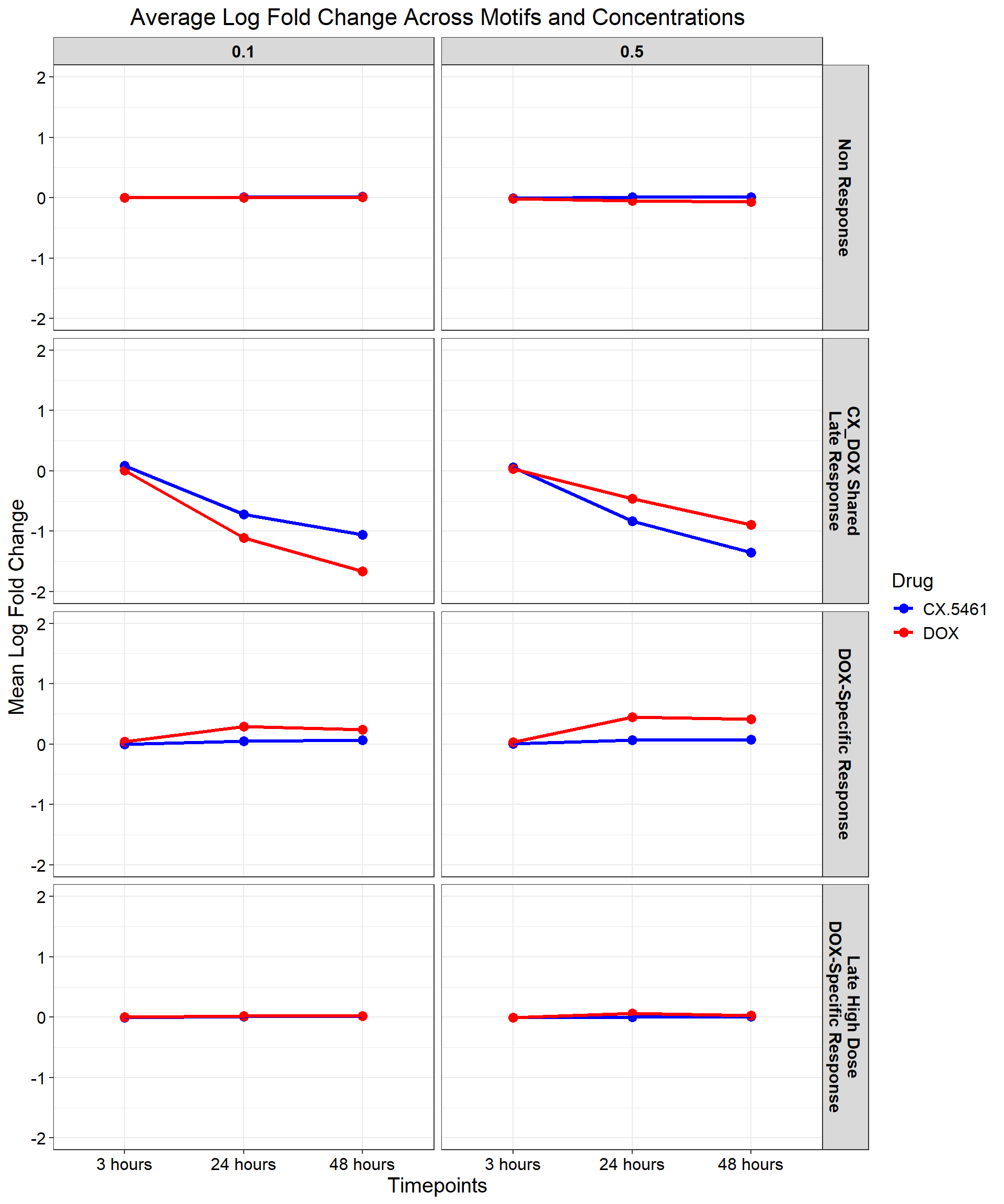
| Version | Author | Date |
|---|---|---|
| 2862c42 | sayanpaul01 | 2025-02-24 |
📌 Save Corr-motif datasets for Gene Ontology analysis
write.csv(data.frame(Entrez_ID = prob_all_1), "data/prob_all_1.csv", row.names = FALSE)
write.csv(data.frame(Entrez_ID = prob_all_2), "data/prob_all_2.csv", row.names = FALSE)
write.csv(data.frame(Entrez_ID = prob_all_3), "data/prob_all_3.csv", row.names = FALSE)
write.csv(data.frame(Entrez_ID = prob_all_4), "data/prob_all_4.csv", row.names = FALSE)
sessionInfo()R version 4.3.0 (2023-04-21 ucrt)
Platform: x86_64-w64-mingw32/x64 (64-bit)
Running under: Windows 11 x64 (build 22631)
Matrix products: default
locale:
[1] LC_COLLATE=English_United States.utf8
[2] LC_CTYPE=English_United States.utf8
[3] LC_MONETARY=English_United States.utf8
[4] LC_NUMERIC=C
[5] LC_TIME=English_United States.utf8
time zone: America/Chicago
tzcode source: internal
attached base packages:
[1] stats4 stats graphics grDevices utils datasets methods
[8] base
other attached packages:
[1] BiocParallel_1.36.0 Rfast_2.1.0 RcppParallel_5.1.9
[4] RcppZiggurat_0.1.6 Rcpp_1.0.12 Cormotif_1.48.0
[7] limma_3.58.1 affy_1.80.0 corrplot_0.95
[10] ggpubr_0.6.0 pheatmap_1.0.12 gprofiler2_0.2.3
[13] RColorBrewer_1.1-3 org.Hs.eg.db_3.18.0 AnnotationDbi_1.64.1
[16] IRanges_2.36.0 S4Vectors_0.40.1 Biobase_2.62.0
[19] BiocGenerics_0.48.1 clusterProfiler_4.10.1 reshape2_1.4.4
[22] lubridate_1.9.3 forcats_1.0.0 stringr_1.5.1
[25] dplyr_1.1.4 purrr_1.0.2 readr_2.1.5
[28] tidyr_1.3.1 tibble_3.2.1 ggplot2_3.5.1
[31] tidyverse_2.0.0 workflowr_1.7.1
loaded via a namespace (and not attached):
[1] rstudioapi_0.17.1 jsonlite_1.8.9 magrittr_2.0.3
[4] farver_2.1.2 rmarkdown_2.29 fs_1.6.3
[7] zlibbioc_1.48.0 vctrs_0.6.5 memoise_2.0.1
[10] RCurl_1.98-1.13 ggtree_3.10.1 rstatix_0.7.2
[13] htmltools_0.5.8.1 broom_1.0.7 Formula_1.2-5
[16] gridGraphics_0.5-1 sass_0.4.9 bslib_0.8.0
[19] htmlwidgets_1.6.4 plyr_1.8.9 plotly_4.10.4
[22] cachem_1.0.8 whisker_0.4.1 igraph_2.1.1
[25] lifecycle_1.0.4 pkgconfig_2.0.3 Matrix_1.6-1.1
[28] R6_2.5.1 fastmap_1.1.1 gson_0.1.0
[31] GenomeInfoDbData_1.2.11 digest_0.6.34 aplot_0.2.3
[34] enrichplot_1.22.0 colorspace_2.1-0 patchwork_1.3.0
[37] ps_1.8.1 rprojroot_2.0.4 RSQLite_2.3.3
[40] labeling_0.4.3 timechange_0.3.0 abind_1.4-8
[43] httr_1.4.7 polyclip_1.10-7 compiler_4.3.0
[46] bit64_4.0.5 withr_3.0.2 backports_1.5.0
[49] carData_3.0-5 viridis_0.6.5 DBI_1.2.3
[52] ggforce_0.4.2 ggsignif_0.6.4 MASS_7.3-60
[55] HDO.db_0.99.1 tools_4.3.0 ape_5.8
[58] scatterpie_0.2.4 httpuv_1.6.15 glue_1.7.0
[61] callr_3.7.6 nlme_3.1-166 GOSemSim_2.28.1
[64] promises_1.3.0 grid_4.3.0 shadowtext_0.1.4
[67] getPass_0.2-4 fgsea_1.28.0 generics_0.1.3
[70] gtable_0.3.6 tzdb_0.4.0 preprocessCore_1.64.0
[73] data.table_1.14.10 hms_1.1.3 car_3.1-3
[76] tidygraph_1.3.1 XVector_0.42.0 ggrepel_0.9.6
[79] pillar_1.10.1 yulab.utils_0.1.8 later_1.3.2
[82] splines_4.3.0 tweenr_2.0.3 treeio_1.26.0
[85] lattice_0.22-5 bit_4.0.5 tidyselect_1.2.1
[88] GO.db_3.18.0 Biostrings_2.70.1 knitr_1.49
[91] git2r_0.35.0 gridExtra_2.3 xfun_0.50
[94] graphlayouts_1.2.0 statmod_1.5.0 stringi_1.8.3
[97] lazyeval_0.2.2 ggfun_0.1.8 yaml_2.3.10
[100] evaluate_1.0.3 codetools_0.2-20 ggraph_2.2.1
[103] qvalue_2.34.0 BiocManager_1.30.25 affyio_1.72.0
[106] ggplotify_0.1.2 cli_3.6.1 munsell_0.5.1
[109] processx_3.8.5 jquerylib_0.1.4 GenomeInfoDb_1.38.8
[112] png_0.1-8 parallel_4.3.0 blob_1.2.4
[115] DOSE_3.28.2 bitops_1.0-7 viridisLite_0.4.2
[118] tidytree_0.4.6 scales_1.3.0 crayon_1.5.3
[121] rlang_1.1.3 cowplot_1.1.3 fastmatch_1.1-4
[124] KEGGREST_1.42.0