Colorectal cancer dataset comparison

workflowr

• Summary
• Checks
• Past versions

Last updated: 2025-06-08

Checks: 6 1

Knit directory: CX5461_Project/

This reproducible R Markdown analysis was created with workflowr (version 1.7.1). The Checks tab describes the reproducibility checks that were applied when the results were created. The Past versions tab lists the development history.

---

R Markdown file: uncommitted changes

The R Markdown file has unstaged changes. To know which version of the R Markdown file created these results, you’ll want to first commit it to the Git repo. If you’re still working on the analysis, you can ignore this warning. When you’re finished, you can run wflow_publish to commit the R Markdown file and build the HTML.

Environment: empty

Great job! The global environment was empty. Objects defined in the global environment can affect the analysis in your R Markdown file in unknown ways. For reproduciblity it’s best to always run the code in an empty environment.

Seed: set.seed(20250129)

The command set.seed(20250129) was run prior to running the code in the R Markdown file. Setting a seed ensures that any results that rely on randomness, e.g. subsampling or permutations, are reproducible.

Session information: recorded

Great job! Recording the operating system, R version, and package versions is critical for reproducibility.

Cache: none

Nice! There were no cached chunks for this analysis, so you can be confident that you successfully produced the results during this run.

File paths: relative

Great job! Using relative paths to the files within your workflowr project makes it easier to run your code on other machines.

Repository version: 044878a

Great! You are using Git for version control. Tracking code development and connecting the code version to the results is critical for reproducibility.

The results in this page were generated with repository version 044878a. See the Past versions tab to see a history of the changes made to the R Markdown and HTML files.

Note that you need to be careful to ensure that all relevant files for the analysis have been committed to Git prior to generating the results (you can use wflow_publish or wflow_git_commit). workflowr only checks the R Markdown file, but you know if there are other scripts or data files that it depends on. Below is the status of the Git repository when the results were generated:

Ignored files:
    Ignored:    .RData
    Ignored:    .Rhistory
    Ignored:    .Rproj.user/
    Ignored:    0.1 box.svg
    Ignored:    Rplot04.svg

Untracked files:
    Untracked:  0.1 density.svg
    Untracked:  0.1.emf
    Untracked:  0.1.svg
    Untracked:  0.5 box.svg
    Untracked:  0.5 density.svg
    Untracked:  0.5.svg
    Untracked:  Additional/
    Untracked:  Autosome factors.svg
    Untracked:  CX_5461_Pattern_Genes_24hr.csv
    Untracked:  CX_5461_Pattern_Genes_3hr.csv
    Untracked:  Cell viability box plot.svg
    Untracked:  DEG GO terms.svg
    Untracked:  DNA damage associated GO terms.svg
    Untracked:  DRC1.svg
    Untracked:  Figure 1.jpeg
    Untracked:  Figure 1.pdf
    Untracked:  Figure_CM_Purity.pdf
    Untracked:  G Quadruplex DEGs.svg
    Untracked:  PC2 Vs PC3 Autosome.svg
    Untracked:  PCA autosome.svg
    Untracked:  Rplot 18.svg
    Untracked:  Rplot.svg
    Untracked:  Rplot01.svg
    Untracked:  Rplot02.svg
    Untracked:  Rplot03.svg
    Untracked:  Rplot05.svg
    Untracked:  Rplot06.svg
    Untracked:  Rplot07.svg
    Untracked:  Rplot08.jpeg
    Untracked:  Rplot08.svg
    Untracked:  Rplot09.svg
    Untracked:  Rplot10.svg
    Untracked:  Rplot11.svg
    Untracked:  Rplot12.svg
    Untracked:  Rplot13.svg
    Untracked:  Rplot14.svg
    Untracked:  Rplot15.svg
    Untracked:  Rplot16.svg
    Untracked:  Rplot17.svg
    Untracked:  Rplot18.svg
    Untracked:  Rplot19.svg
    Untracked:  Rplot20.svg
    Untracked:  Rplot21.svg
    Untracked:  Rplot22.svg
    Untracked:  Rplot23.svg
    Untracked:  Rplot24.svg
    Untracked:  TOP2B.bed
    Untracked:  TS HPA (Violin).svg
    Untracked:  TS HPA.svg
    Untracked:  TS_HA.svg
    Untracked:  TS_HV.svg
    Untracked:  Violin HA.svg
    Untracked:  Violin HV (CX vs DOX).svg
    Untracked:  Violin HV.svg
    Untracked:  data/AF.csv
    Untracked:  data/AF_Mapped.csv
    Untracked:  data/AF_genes.csv
    Untracked:  data/Annotated_DOX_Gene_Table.csv
    Untracked:  data/BP/
    Untracked:  data/CAD_genes.csv
    Untracked:  data/Cardiotox.csv
    Untracked:  data/Cardiotox_mapped.csv
    Untracked:  data/Col_DEGs.csv
    Untracked:  data/Corrmotif_GO/
    Untracked:  data/DOX_Vald.csv
    Untracked:  data/DOX_Vald_Mapped.csv
    Untracked:  data/DOX_alt.csv
    Untracked:  data/Entrez_Cardiotox.csv
    Untracked:  data/Entrez_Cardiotox_Mapped.csv
    Untracked:  data/GWAS.xlsx
    Untracked:  data/GWAS_SNPs.bed
    Untracked:  data/HF.csv
    Untracked:  data/HF_Mapped.csv
    Untracked:  data/HF_genes.csv
    Untracked:  data/Hypertension_genes.csv
    Untracked:  data/MI_genes.csv
    Untracked:  data/P53_Target_mapped.csv
    Untracked:  data/Sample_annotated.csv
    Untracked:  data/Samples.csv
    Untracked:  data/Samples.xlsx
    Untracked:  data/TOP2A.bed
    Untracked:  data/TOP2A_target.csv
    Untracked:  data/TOP2A_target_lit.csv
    Untracked:  data/TOP2A_target_lit_mapped.csv
    Untracked:  data/TOP2A_target_mapped.csv
    Untracked:  data/TOP2B.bed
    Untracked:  data/TOP2B_target.csv
    Untracked:  data/TOP2B_target_heatmap.csv
    Untracked:  data/TOP2B_target_heatmap_mapped.csv
    Untracked:  data/TOP2B_target_mapped.csv
    Untracked:  data/TS.csv
    Untracked:  data/TS_HPA.csv
    Untracked:  data/TS_HPA_mapped.csv
    Untracked:  data/Toptable_CX_0.1_24.csv
    Untracked:  data/Toptable_CX_0.1_3.csv
    Untracked:  data/Toptable_CX_0.1_48.csv
    Untracked:  data/Toptable_CX_0.5_24.csv
    Untracked:  data/Toptable_CX_0.5_3.csv
    Untracked:  data/Toptable_CX_0.5_48.csv
    Untracked:  data/Toptable_DOX_0.1_24.csv
    Untracked:  data/Toptable_DOX_0.1_3.csv
    Untracked:  data/Toptable_DOX_0.1_48.csv
    Untracked:  data/Toptable_DOX_0.5_24.csv
    Untracked:  data/Toptable_DOX_0.5_3.csv
    Untracked:  data/Toptable_DOX_0.5_48.csv
    Untracked:  data/count.tsv
    Untracked:  data/heatmap.csv
    Untracked:  data/ts_data_mapped
    Untracked:  results/
    Untracked:  run_bedtools.bat

Unstaged changes:
    Deleted:    analysis/Actox.Rmd
    Modified:   analysis/Colorectal.Rmd
    Modified:   data/DOX_0.5_48 (Combined).csv
    Modified:   data/Human_Heart_Genes.csv
    Modified:   data/Total_number_of_Mapped_reads_by_Individuals.csv

Note that any generated files, e.g. HTML, png, CSS, etc., are not included in this status report because it is ok for generated content to have uncommitted changes.

---

These are the previous versions of the repository in which changes were made to the R Markdown (analysis/Colorectal.Rmd) and HTML (docs/Colorectal.html) files. If you’ve configured a remote Git repository (see ?wflow_git_remote), click on the hyperlinks in the table below to view the files as they were in that past version.

File	Version	Author	Date	Message
Rmd	488c5c4	sayanpaul01	2025-06-02	Commit
html	488c5c4	sayanpaul01	2025-06-02	Commit
Rmd	ffaf948	sayanpaul01	2025-04-06	Commit
html	491cd15	sayanpaul01	2025-03-30	Commit
Rmd	bf87a05	sayanpaul01	2025-03-30	Commit
html	bf87a05	sayanpaul01	2025-03-30	Commit
Rmd	0649bff	sayanpaul01	2025-03-30	Commit
html	0649bff	sayanpaul01	2025-03-30	Commit
Rmd	44d47e5	sayanpaul01	2025-03-16	Commit
html	44d47e5	sayanpaul01	2025-03-16	Commit
html	ef3a951	sayanpaul01	2025-03-09	Commit
Rmd	0aec578	sayanpaul01	2025-03-06	Commit
html	0aec578	sayanpaul01	2025-03-06	Commit
Rmd	3e51d79	sayanpaul01	2025-03-05	Commit
html	3e51d79	sayanpaul01	2025-03-05	Commit
Rmd	1c452e8	sayanpaul01	2025-03-05	Commit
html	1c452e8	sayanpaul01	2025-03-05	Commit
Rmd	5b6c285	sayanpaul01	2025-02-28	Commit
html	5b6c285	sayanpaul01	2025-02-28	Commit
Rmd	1c1e1e4	sayanpaul01	2025-02-28	Commit
html	1c1e1e4	sayanpaul01	2025-02-28	Commit

---

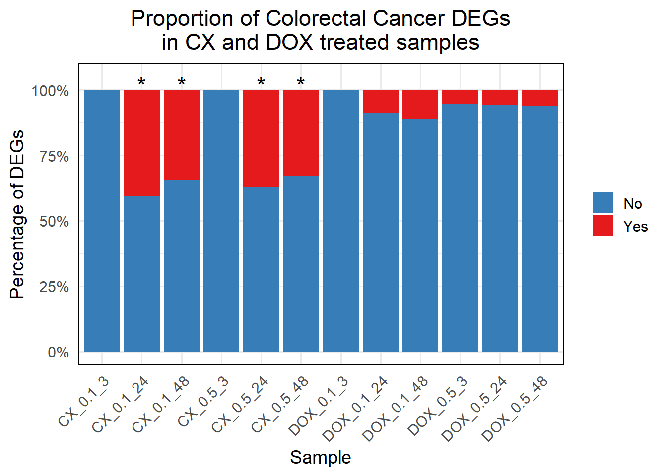
📌 Proportion of Colorectal cancer DEGs in CX and DOX treated samples

📌 Load Required Libraries

# 📦 Load Required Libraries
# 📦 Load Required Libraries
library(tidyverse)

Warning: package 'tidyverse' was built under R version 4.3.2

Warning: package 'tidyr' was built under R version 4.3.3

Warning: package 'readr' was built under R version 4.3.3

Warning: package 'purrr' was built under R version 4.3.3

Warning: package 'dplyr' was built under R version 4.3.2

Warning: package 'stringr' was built under R version 4.3.2

Warning: package 'lubridate' was built under R version 4.3.3

library(org.Hs.eg.db)

Warning: package 'AnnotationDbi' was built under R version 4.3.2

Warning: package 'BiocGenerics' was built under R version 4.3.1

Warning: package 'Biobase' was built under R version 4.3.1

Warning: package 'IRanges' was built under R version 4.3.1

Warning: package 'S4Vectors' was built under R version 4.3.2

# 📁 Load Consolidated Gene Symbols and convert to Entrez
col_symbols <- read.csv("data/Col_DEGs.csv") %>%
  pull(Symbol) %>%
  unique()

col_entrez <- mapIds(
  org.Hs.eg.db,
  keys = col_symbols,
  column = "ENTREZID",
  keytype = "SYMBOL",
  multiVals = "first"
) %>%
  na.omit() %>%
  unique() %>%
  as.character()

# 🧬 Load DEG Data
deg_list <- list(
  "CX_0.1_3"   = read.csv("data/DEGs/Toptable_CX_0.1_3.csv"),
  "CX_0.1_24"  = read.csv("data/DEGs/Toptable_CX_0.1_24.csv"),
  "CX_0.1_48"  = read.csv("data/DEGs/Toptable_CX_0.1_48.csv"),
  "CX_0.5_3"   = read.csv("data/DEGs/Toptable_CX_0.5_3.csv"),
  "CX_0.5_24"  = read.csv("data/DEGs/Toptable_CX_0.5_24.csv"),
  "CX_0.5_48"  = read.csv("data/DEGs/Toptable_CX_0.5_48.csv"),
  "DOX_0.1_3"  = read.csv("data/DEGs/Toptable_DOX_0.1_3.csv"),
  "DOX_0.1_24" = read.csv("data/DEGs/Toptable_DOX_0.1_24.csv"),
  "DOX_0.1_48" = read.csv("data/DEGs/Toptable_DOX_0.1_48.csv"),
  "DOX_0.5_3"  = read.csv("data/DEGs/Toptable_DOX_0.5_3.csv"),
  "DOX_0.5_24" = read.csv("data/DEGs/Toptable_DOX_0.5_24.csv"),
  "DOX_0.5_48" = read.csv("data/DEGs/Toptable_DOX_0.5_48.csv")
)

# ✅ Extract Significant DEGs and Calculate Overlap
proportion_data <- map_dfr(names(deg_list), function(sample) {
  sig_df <- deg_list[[sample]] %>%
    filter(adj.P.Val < 0.05)
  sample_degs <- unique(as.character(sig_df$Entrez_ID))
  
  yes <- sum(sample_degs %in% col_entrez)
  no <- length(sample_degs) - yes
  
  data.frame(
    Sample = sample,
    Category = c("Yes", "No"),
    Count = c(yes, no)
  )
}) %>%
  group_by(Sample) %>%
  mutate(Proportion = Count / sum(Count) * 100)

# 🔁 Reorder Sample Levels
proportion_data$Sample <- factor(proportion_data$Sample, levels = c(
  "CX_0.1_3", "CX_0.1_24", "CX_0.1_48",
  "CX_0.5_3", "CX_0.5_24", "CX_0.5_48",
  "DOX_0.1_3", "DOX_0.1_24", "DOX_0.1_48",
  "DOX_0.5_3", "DOX_0.5_24", "DOX_0.5_48"
))

# ✅ Set Yes on top
proportion_data$Category <- factor(proportion_data$Category, levels = c("Yes", "No"))

# 🔬 Chi-square Test for CX vs DOX matched conditions
matched_pairs <- list(
  "0.1_3"  = c("CX_0.1_3", "DOX_0.1_3"),
  "0.1_24" = c("CX_0.1_24", "DOX_0.1_24"),
  "0.1_48" = c("CX_0.1_48", "DOX_0.1_48"),
  "0.5_3"  = c("CX_0.5_3", "DOX_0.5_3"),
  "0.5_24" = c("CX_0.5_24", "DOX_0.5_24"),
  "0.5_48" = c("CX_0.5_48", "DOX_0.5_48")
)

# Compute p-values
chi_results <- map_dfr(names(matched_pairs), function(label) {
  cx <- matched_pairs[[label]][1]
  dox <- matched_pairs[[label]][2]
  
  cx_df <- deg_list[[cx]] %>% filter(adj.P.Val < 0.05)
  dox_df <- deg_list[[dox]] %>% filter(adj.P.Val < 0.05)
  
  a1 <- sum(cx_df$Entrez_ID %in% col_entrez)
  b1 <- nrow(cx_df) - a1
  a2 <- sum(dox_df$Entrez_ID %in% col_entrez)
  b2 <- nrow(dox_df) - a2
  
  chisq <- chisq.test(matrix(c(a1, b1, a2, b2), nrow = 2, byrow = TRUE))
  
  data.frame(
    Comparison = label,
    CX_sample = cx,
    DOX_sample = dox,
    P_value = chisq$p.value,
    Star = ifelse(chisq$p.value < 0.05, "*", "")
  )
})

Warning in chisq.test(matrix(c(a1, b1, a2, b2), nrow = 2, byrow = TRUE)):
Chi-squared approximation may be incorrect

Warning in chisq.test(matrix(c(a1, b1, a2, b2), nrow = 2, byrow = TRUE)):
Chi-squared approximation may be incorrect

# ✏️ Label placement
# 🆙 Place stars only above CX samples where p < 0.05
# Ensure dplyr functions are used explicitly
annot_df <- chi_results %>%
  dplyr::filter(Star == "*") %>%
  dplyr::select(CX_sample, Star) %>%
  dplyr::rename(Sample = CX_sample) %>%
  dplyr::mutate(y_pos = 102)



ggplot(proportion_data, aes(x = Sample, y = Proportion, fill = Category)) +
  geom_bar(stat = "identity", position = "stack") +
  geom_text(data = annot_df, aes(x = Sample, y = y_pos, label = Star),
            inherit.aes = FALSE, size = 6) +
  scale_fill_manual(
    values = c("Yes" = "#e41a1c", "No" = "#377eb8"),
    guide = guide_legend(reverse = TRUE)
  ) +
  scale_y_continuous(labels = scales::percent_format(scale = 1), limits = c(0, 105)) +
  labs(
    title = "Proportion of Colorectal Cancer DEGs\nin CX and DOX treated samples",
    x = "Sample",
    y = "Percentage of DEGs",
    fill = "Overlap"
  ) +
  theme_minimal(base_size = 14) +
  theme(
    axis.text.x = element_text(angle = 45, hjust = 1),
    plot.title = element_text(hjust = 0.5),
    legend.title = element_blank(),
    panel.border = element_rect(color = "black", fill = NA, linewidth = 1)
  )

📌 Proportion of Colorectal cancer DE genes in Corrmotif clusters

📌 Load Required Libraries

library(ggplot2)
library(dplyr)
library(tidyr)
library(org.Hs.eg.db)
library(clusterProfiler)

Warning: package 'clusterProfiler' was built under R version 4.3.3

library(biomaRt)

Warning: package 'biomaRt' was built under R version 4.3.2

📌 Load Data

# Define correct timepoints
timepoints <- c("6hr", "24hr", "72hr")

# Initialize an empty dataframe to store chi-square results
all_chi_results <- data.frame()

# Loop through each timepoint and perform Chi-square test
for (time in timepoints) {
  
  # Load proportion data for the given timepoint
  file_path <- paste0("data/Colorectal/Proportion_data_", time, ".csv")
  
  # Check if the file exists before reading
  if (!file.exists(file_path)) {
    cat("\n🚨 Warning: File does not exist:", file_path, "\nSkipping this timepoint...\n")
    next  # Skip this iteration if the file is missing
  }
  
  proportion_data <- read.csv(file_path)
  
  # Extract counts for Non-Response group
  non_response_counts <- proportion_data %>%
    filter(Set == "Non Response") %>%
    dplyr::select(DEG, `Non.DEG`) %>%
    unlist(use.names = FALSE)  # Convert to numeric vector
  
  # Debugging: Print Non-Response counts
  cat("\nNon-Response Counts for", time, ":\n")
  print(non_response_counts)
  
  # Initialize a list to store chi-square test results for this timepoint
  chi_results <- list()
  
  # Perform chi-square test for each response group
  for (group in unique(proportion_data$Set)) {
    if (group == "Non Response") next  # Skip Non Response group
    
    # Extract counts for the current response group
    group_counts <- proportion_data %>%
      filter(Set == group) %>%
      dplyr::select(DEG, `Non.DEG`) %>%
      unlist(use.names = FALSE)  # Convert to numeric vector
    
    # Ensure valid counts for chi-square test
    if (length(group_counts) < 2) group_counts <- c(group_counts, 0)
    if (length(non_response_counts) < 2) non_response_counts <- c(non_response_counts, 0)
    
    # Create contingency table
    contingency_table <- matrix(c(
      group_counts[1], group_counts[2],  # Current response group counts
      non_response_counts[1], non_response_counts[2]  # Non-Response counts
    ), nrow = 2, byrow = TRUE)
    
    # Debugging: Print contingency table
    cat("\nProcessing Group:", group, "at", time, "\n")
    cat("Contingency Table:\n")
    print(contingency_table)
    
    # Perform chi-square test
    test_result <- chisq.test(contingency_table)
    p_value <- test_result$p.value
    significance <- ifelse(p_value < 0.05, "*", "")  # Mark * for p < 0.05
    
    # Store results
    chi_results[[group]] <- data.frame(
      Set = group,
      Timepoint = time,
      Chi2 = test_result$statistic,
      p_value = p_value,
      Significance = significance
    )
  }
  
  # Combine results for this timepoint into a single dataframe
  chi_results <- do.call(rbind, chi_results)
  
  # Append to the overall results dataframe
  all_chi_results <- rbind(all_chi_results, chi_results)
}

# Save final chi-square results
write.csv(all_chi_results, "data/Colorectal//Chi_Square_Results_All.csv", row.names = FALSE)

📌 Proportion of DE genes across response groups

# Load the saved datasets
prob_all_1 <- read.csv("data/prob_all_1.csv")$Entrez_ID
prob_all_2 <- read.csv("data/prob_all_2.csv")$Entrez_ID
prob_all_3 <- read.csv("data/prob_all_3.csv")$Entrez_ID
prob_all_4 <- read.csv("data/prob_all_4.csv")$Entrez_ID

# Example Response Groups Data (Replace with actual data)
response_groups <- list(
  "Non Response" = prob_all_1, # Replace 'prob_all_1', 'prob_all_2', etc. with your actual response group dataframes
  "CX_DOX Shared Late Response" = prob_all_2,
  "DOX-Specific Response" = prob_all_3,
  "Late High Dose DOX-Specific Response" = prob_all_4
)

# Load the proportion data again for visualization
proportion_data <-read.csv("data/Colorectal/Proportion_data.csv")
# Merge chi-square results into proportion data for plotting
proportion_data <- proportion_data %>%
  left_join(all_chi_results %>% dplyr::select(Set, Timepoint, Significance), by = c("Set", "Timepoint"))

# Convert to factors for ordered display
proportion_data$Set <- factor(proportion_data$Set, levels = c(
  "Non Response",
  "CX_DOX Shared Late Response",
  "DOX-Specific Response",
  "Late High Dose DOX-Specific Response"
))
proportion_data$Timepoint <- factor(proportion_data$Timepoint, levels = timepoints)

# Plot proportions with significance stars
ggplot(proportion_data, aes(x = Set, y = Percentage, fill = Category)) +
  geom_bar(stat = "identity", position = "stack") +
  facet_wrap(~Timepoint, scales = "fixed") +
  scale_fill_manual(values = c("DEG" = "#e41a1c", "Non-DEG" = "#377eb8")) +
  geom_text(
    data = proportion_data %>% filter(Significance == "*") %>% distinct(Set, Timepoint, Significance),
    aes(x = Set, y = 105, label = Significance),
    inherit.aes = FALSE,
    size = 6,
    color = "black",
    hjust = 0.5
  ) +
  labs(
    title = "Proportion of Colorectal cancer DEGs and Non-DEGs\nAcross Response Groups (6hr, 24hr, 72hr)",
    x = "Response Groups",
    y = "Percentage",
    fill = "Category"
  ) +
  theme_minimal() +
  theme(
    plot.title = element_text(size = rel(1.5), hjust = 0.5),
    axis.title = element_text(size = 15, color = "black"),
    axis.text.x = element_text(size = 10, angle = 45, hjust = 1),
    legend.title = element_blank(),
    panel.border = element_rect(color = "black", fill = NA, size = 1.2),
    strip.background = element_blank(),
    strip.text = element_text(size = 12, face = "bold")
  )

Warning: The `size` argument of `element_rect()` is deprecated as of ggplot2 3.4.0.
ℹ Please use the `linewidth` argument instead.
This warning is displayed once every 8 hours.
Call `lifecycle::last_lifecycle_warnings()` to see where this warning was
generated.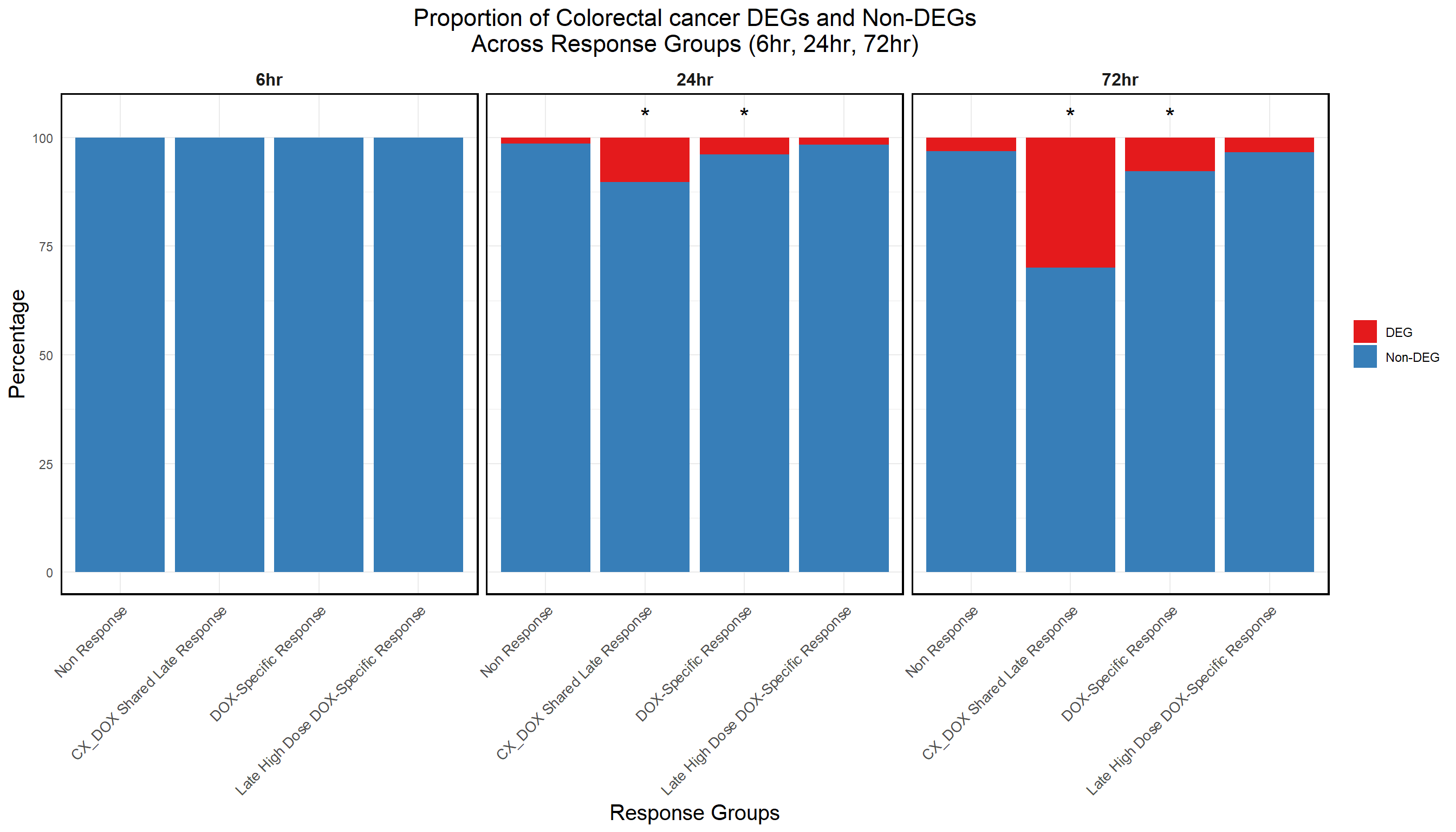

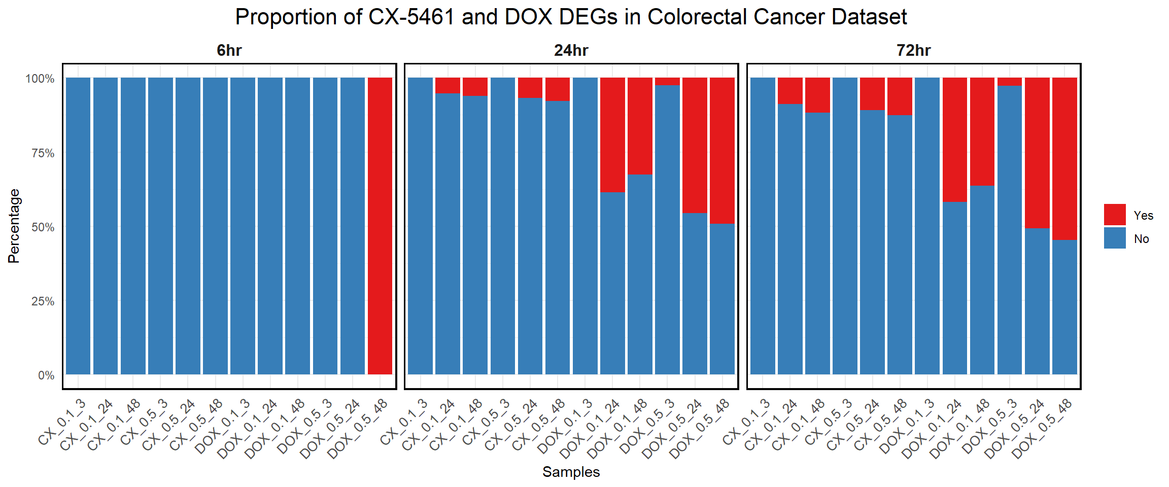
Past versions of load_data_tissue-1.png

Version	Author	Date
0649bff	sayanpaul01	2025-03-30
1c1e1e4	sayanpaul01	2025-02-28

📌 Proportion of CX and DOX DEGs in colorectal cancer genes

📌 Read and Process Data

# Load necessary libraries
library(dplyr)
library(ggplot2)
library(tidyr)
library(org.Hs.eg.db)

# Load DEGs Data
CX_0.1_3 <- read.csv("data/DEGs/Toptable_CX_0.1_3.csv")
CX_0.1_24 <- read.csv("data/DEGs/Toptable_CX_0.1_24.csv")
CX_0.1_48 <- read.csv("data/DEGs/Toptable_CX_0.1_48.csv")
CX_0.5_3 <- read.csv("data/DEGs/Toptable_CX_0.5_3.csv")
CX_0.5_24 <- read.csv("data/DEGs/Toptable_CX_0.5_24.csv")
CX_0.5_48 <- read.csv("data/DEGs/Toptable_CX_0.5_48.csv")

DOX_0.1_3 <- read.csv("data/DEGs/Toptable_DOX_0.1_3.csv")
DOX_0.1_24 <- read.csv("data/DEGs/Toptable_DOX_0.1_24.csv")
DOX_0.1_48 <- read.csv("data/DEGs/Toptable_DOX_0.1_48.csv")
DOX_0.5_3 <- read.csv("data/DEGs/Toptable_DOX_0.5_3.csv")
DOX_0.5_24 <- read.csv("data/DEGs/Toptable_DOX_0.5_24.csv")
DOX_0.5_48 <- read.csv("data/DEGs/Toptable_DOX_0.5_48.csv")

# Extract Significant DEGs
extract_DEGs <- function(df) as.character(df$Entrez_ID[df$adj.P.Val < 0.05])

CX_DEGs <- list(
  "CX_0.1_3" = extract_DEGs(CX_0.1_3), "CX_0.1_24" = extract_DEGs(CX_0.1_24), "CX_0.1_48" = extract_DEGs(CX_0.1_48),
  "CX_0.5_3" = extract_DEGs(CX_0.5_3), "CX_0.5_24" = extract_DEGs(CX_0.5_24), "CX_0.5_48" = extract_DEGs(CX_0.5_48)
)

DOX_DEGs <- list(
  "DOX_0.1_3" = extract_DEGs(DOX_0.1_3), "DOX_0.1_24" = extract_DEGs(DOX_0.1_24), "DOX_0.1_48" = extract_DEGs(DOX_0.1_48),
  "DOX_0.5_3" = extract_DEGs(DOX_0.5_3), "DOX_0.5_24" = extract_DEGs(DOX_0.5_24), "DOX_0.5_48" = extract_DEGs(DOX_0.5_48)
)

# Load Colorectal Cancer Gene Lists
data_6hr <- read.csv("data/Colorectal/6hr.csv", stringsAsFactors = FALSE)
data_24hr <- read.csv("data/Colorectal/24hr.csv", stringsAsFactors = FALSE)
data_72hr <- read.csv("data/Colorectal/72hr.csv", stringsAsFactors = FALSE)

# Convert Gene Symbols to Entrez IDs
data_list <- list("6hr" = data_6hr, "24hr" = data_24hr, "72hr" = data_72hr)
data_list <- lapply(data_list, function(df) {
  df %>% mutate(Entrez_ID = mapIds(org.Hs.eg.db, keys = Symbol, column = "ENTREZID", keytype = "SYMBOL", multiVals = "first")) %>% na.omit()
})

lit_genes <- lapply(data_list, function(df) df$Entrez_ID)

# Function to calculate DEGs proportion in Colorectal Cancer dataset
calculate_proportion <- function(deg_list, drug_name, cancer_genes, timepoint) {
  data.frame(
    Sample = names(deg_list),
    Drug = drug_name,
    Timepoint = timepoint,
    DEGs_in_Cancer = sapply(deg_list, function(ids) sum(ids %in% cancer_genes)),
    Non_DEGs_in_Cancer = length(cancer_genes) - sapply(deg_list, function(ids) sum(ids %in% cancer_genes))
  ) %>%
    mutate(
      Yes_Proportion = (DEGs_in_Cancer / length(cancer_genes)) * 100,
      No_Proportion = (Non_DEGs_in_Cancer / length(cancer_genes)) * 100
    )
}

# Calculate Proportions for Each Timepoint
proportion_data <- bind_rows(
  lapply(names(lit_genes), function(tp) calculate_proportion(CX_DEGs, "CX-5461", lit_genes[[tp]], tp)),
  lapply(names(lit_genes), function(tp) calculate_proportion(DOX_DEGs, "DOX", lit_genes[[tp]], tp))
)

# Convert Data to Long Format for Faceting
proportion_long <- proportion_data %>%
  pivot_longer(cols = c(Yes_Proportion, No_Proportion), names_to = "Category", values_to = "Percentage") %>%
  mutate(Category = ifelse(Category == "Yes_Proportion", "Yes", "No"))

# Ensure Correct Ordering
sample_order <- c(
  "CX_0.1_3", "CX_0.1_24", "CX_0.1_48", "CX_0.5_3", "CX_0.5_24", "CX_0.5_48",
  "DOX_0.1_3", "DOX_0.1_24", "DOX_0.1_48", "DOX_0.5_3", "DOX_0.5_24", "DOX_0.5_48"
)
proportion_long$Sample <- factor(proportion_long$Sample, levels = sample_order)
proportion_long$Timepoint <- factor(proportion_long$Timepoint, levels = c("6hr", "24hr", "72hr"))
proportion_long$Category <- factor(proportion_long$Category, levels = c("Yes", "No"))

# Generate Stacked Bar Plot with Faceting
ggplot(proportion_long, aes(x = Sample, y = Percentage, fill = Category)) +
  geom_bar(stat = "identity", position = "stack") +
  facet_wrap(~Timepoint, scales = "fixed") +
  scale_y_continuous(labels = scales::percent_format(scale = 1), limits = c(0, 100)) +
  scale_fill_manual(values = c("Yes" = "#e41a1c", "No" = "#377eb8")) +
  labs(
    title = "Proportion of CX-5461 and DOX DEGs in Colorectal Cancer Dataset",
    x = "Samples",
    y = "Percentage",
    fill = "Category"
  ) +
  theme_minimal() +
  theme(
    plot.title = element_text(size = rel(1.5), hjust = 0.5),
    axis.text.x = element_text(size = 10, angle = 45, hjust = 1),
    legend.title = element_blank(),
    panel.border = element_rect(color = "black", fill = NA, linewidth = 1.2),
    strip.background = element_blank(),
    strip.text = element_text(size = 12, face = "bold")
  )

Past versions of load_DEGs-1.png

Version	Author	Date
0649bff	sayanpaul01	2025-03-30
3e51d79	sayanpaul01	2025-03-05
1c452e8	sayanpaul01	2025-03-05

📌 Correlation of colorectal cancer genes with CX and DOX expressed genes

📌 6hr

# Import the CSV file
data_6hr_logFC <- read.csv("data/Colorectal/6hrlogFC.csv", stringsAsFactors = FALSE)

# Map gene symbols to Entrez IDs using org.Hs.eg.db
data_6hr_logFC <- data_6hr_logFC %>%
  mutate(Entrez_ID = mapIds(org.Hs.eg.db,
                            keys = Symbol,
                            column = "ENTREZID",
                            keytype = "SYMBOL",
                            multiVals = "first"))

# Merge datasets on Entrez_ID for CX and DOX at both concentrations (3 hours)
merged_CX_0.1 <- merge(data_6hr_logFC, CX_0.1_3, by = "Entrez_ID")
merged_CX_0.5 <- merge(data_6hr_logFC, CX_0.5_3, by = "Entrez_ID")
merged_DOX_0.1 <- merge(data_6hr_logFC, DOX_0.1_3, by = "Entrez_ID")
merged_DOX_0.5 <- merge(data_6hr_logFC, DOX_0.5_3, by = "Entrez_ID")

# Remove NA values
merged_CX_0.1 <- na.omit(merged_CX_0.1)
merged_CX_0.5 <- na.omit(merged_CX_0.5)
merged_DOX_0.1 <- na.omit(merged_DOX_0.1)
merged_DOX_0.5 <- na.omit(merged_DOX_0.5)

# Rename columns explicitly to avoid conflicts
colnames(merged_CX_0.1) <- colnames(merged_CX_0.5) <-
  colnames(merged_DOX_0.1) <- colnames(merged_DOX_0.5) <-
  c("Entrez_ID", "Symbol_6hr", "logFC_6hr", "logFC_Drug", "AveExpr_Drug", "t_Drug", "P.Value_Drug", "adj.P.Val_Drug", "B_Drug")

# Add drug and concentration labels for faceting
merged_CX_0.1$Drug <- "CX (3hr)"
merged_CX_0.5$Drug <- "CX (3hr)"
merged_DOX_0.1$Drug <- "DOX (3hr)"
merged_DOX_0.5$Drug <- "DOX (3hr)"

merged_CX_0.1$Concentration <- "0.1 µM"
merged_CX_0.5$Concentration <- "0.5 µM"
merged_DOX_0.1$Concentration <- "0.1 µM"
merged_DOX_0.5$Concentration <- "0.5 µM"

# Combine all datasets into a single data frame
merged_data <- rbind(
  merged_CX_0.1[, c("Entrez_ID", "logFC_Drug", "logFC_6hr", "Concentration", "Drug")],
  merged_CX_0.5[, c("Entrez_ID", "logFC_Drug", "logFC_6hr", "Concentration", "Drug")],
  merged_DOX_0.1[, c("Entrez_ID", "logFC_Drug", "logFC_6hr", "Concentration", "Drug")],
  merged_DOX_0.5[, c("Entrez_ID", "logFC_Drug", "logFC_6hr", "Concentration", "Drug")]
)

# Calculate correlations for each facet
cor_CX_0.1 <- cor.test(merged_CX_0.1$logFC_Drug, merged_CX_0.1$logFC_6hr, method = "pearson")
cor_CX_0.5 <- cor.test(merged_CX_0.5$logFC_Drug, merged_CX_0.5$logFC_6hr, method = "pearson")
cor_DOX_0.1 <- cor.test(merged_DOX_0.1$logFC_Drug, merged_DOX_0.1$logFC_6hr, method = "pearson")
cor_DOX_0.5 <- cor.test(merged_DOX_0.5$logFC_Drug, merged_DOX_0.5$logFC_6hr, method = "pearson")

# Data frame for r and p-values annotations
correlation_data <- data.frame(
  Drug = rep(c("CX (3hr)", "DOX (3hr)"), each = 2),
  Concentration = rep(c("0.1 µM", "0.5 µM"), times = 2),
  x = max(merged_data$logFC_Drug, na.rm = TRUE) * 0.75,  # Adjusted placement for better fit
  y = max(merged_data$logFC_6hr, na.rm = TRUE) * 0.85,
  label = c(
    paste0("r = ", round(cor_CX_0.1$estimate, 3), "\np = ", signif(cor_CX_0.1$p.value, 3)),
    paste0("r = ", round(cor_CX_0.5$estimate, 3), "\np = ", signif(cor_CX_0.5$p.value, 3)),
    paste0("r = ", round(cor_DOX_0.1$estimate, 3), "\np = ", signif(cor_DOX_0.1$p.value, 3)),
    paste0("r = ", round(cor_DOX_0.5$estimate, 3), "\np = ", signif(cor_DOX_0.5$p.value, 3))
  )
)

# Create scatter plot with facets for concentration (vertically) and drug (horizontally)
scatter_plot <- ggplot(merged_data, aes(x = logFC_Drug, y = logFC_6hr)) +
  geom_point(alpha = 0.6, color = "black") +  # Black scatter points
  geom_smooth(method = "lm", color = "black", se = FALSE) +  # Black regression line
  labs(
    title = "Correlation between Drug (3hr) and Colorectal 6hr logFC",
    x = "logFC (Drug_3hr)",
    y = "logFC (Colorectal 6hr)"
  ) +
  theme_minimal() +
  theme(
    plot.title = element_text(size = 14, face = "bold"),

    # Outer box around the entire facet plot
    panel.border = element_rect(color = "black", fill = NA, linewidth = 2),

    # Black box around each facet title
    strip.background = element_rect(fill = "white", color = "black", linewidth = 1.5),
    strip.text = element_text(size = 12, face = "bold", color = "black")
  ) +

  # Facet by drug (horizontally) and concentration (vertically)
  facet_grid(Concentration ~ Drug) +

  # Add r and p-value in the upper-right corner of each facet with better fitting font size
  geom_text(data = correlation_data,
            aes(x = x, y = y, label = label),
            inherit.aes = FALSE, size = 3, fontface = "bold")  # Reduced font size for better fit

# Display plot
print(scatter_plot)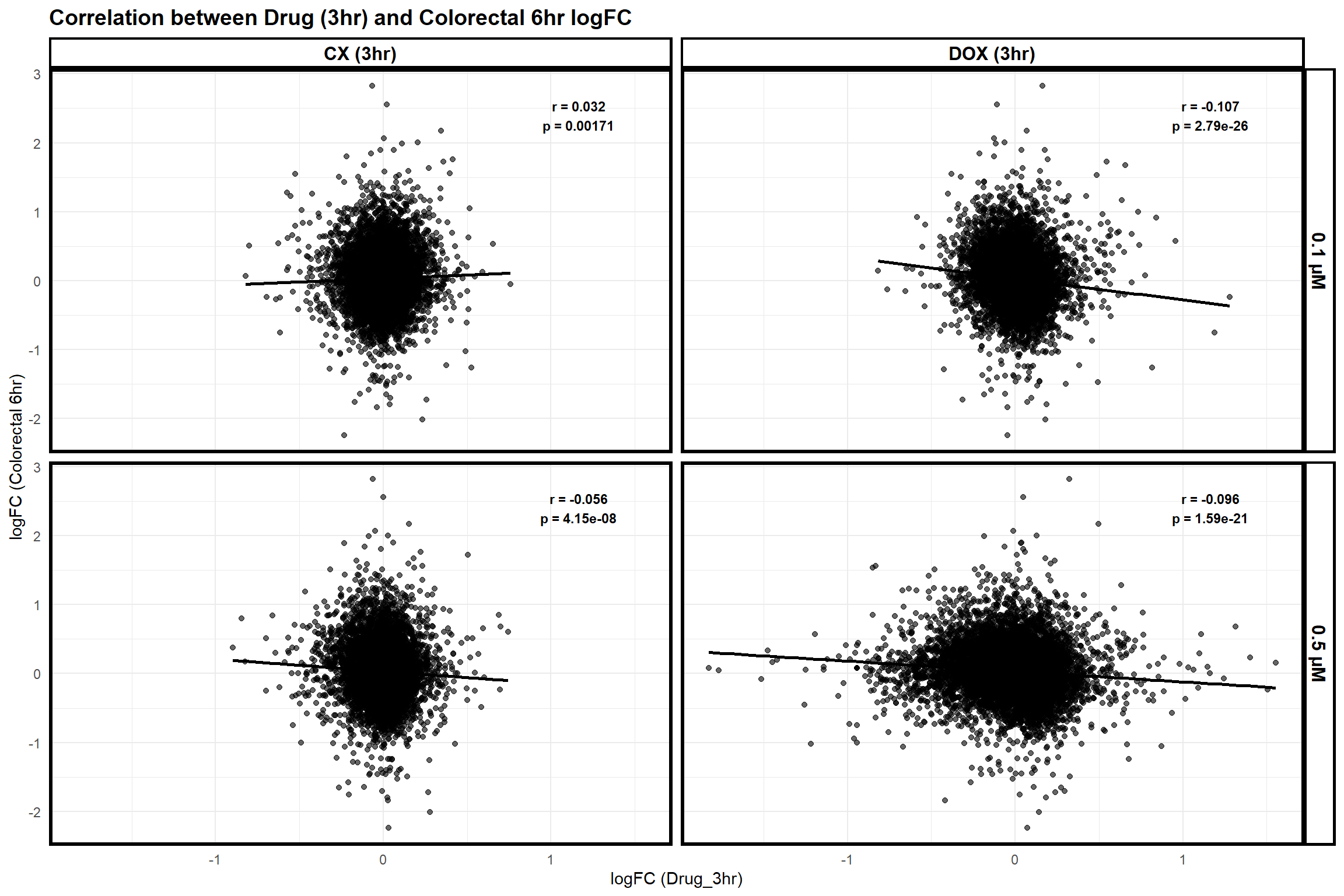

Past versions of Data_prep-1.png

Version	Author	Date
0649bff	sayanpaul01	2025-03-30
5b6c285	sayanpaul01	2025-02-28

📌 24hr

# Import the CSV file
data_24hr_logFC <- read.csv("data/Colorectal/24hrlogFC.csv", stringsAsFactors = FALSE)

# Map gene symbols to Entrez IDs using org.Hs.eg.db
data_24hr_logFC <- data_24hr_logFC %>%
  mutate(Entrez_ID = mapIds(org.Hs.eg.db,
                            keys = Symbol,
                            column = "ENTREZID",
                            keytype = "SYMBOL",
                            multiVals = "first"))

# Merge datasets on Entrez_ID for CX and DOX at both concentrations (24 hours)
merged_CX_0.1_24 <- merge(data_24hr_logFC, CX_0.1_24, by = "Entrez_ID")
merged_CX_0.5_24 <- merge(data_24hr_logFC, CX_0.5_24, by = "Entrez_ID")
merged_DOX_0.1_24 <- merge(data_24hr_logFC, DOX_0.1_24, by = "Entrez_ID")
merged_DOX_0.5_24 <- merge(data_24hr_logFC, DOX_0.5_24, by = "Entrez_ID")

# Remove NA values
merged_CX_0.1_24 <- na.omit(merged_CX_0.1_24)
merged_CX_0.5_24 <- na.omit(merged_CX_0.5_24)
merged_DOX_0.1_24 <- na.omit(merged_DOX_0.1_24)
merged_DOX_0.5_24 <- na.omit(merged_DOX_0.5_24)

# Rename columns explicitly to avoid conflicts
colnames(merged_CX_0.1_24) <- colnames(merged_CX_0.5_24) <-
  colnames(merged_DOX_0.1_24) <- colnames(merged_DOX_0.5_24) <-
  c("Entrez_ID", "Symbol_24hr", "logFC_24hr", "logFC_Drug", "AveExpr_Drug", "t_Drug", "P.Value_Drug", "adj.P.Val_Drug", "B_Drug")

# Add drug and concentration labels for faceting
merged_CX_0.1_24$Drug <- "CX (24hr)"
merged_CX_0.5_24$Drug <- "CX (24hr)"
merged_DOX_0.1_24$Drug <- "DOX (24hr)"
merged_DOX_0.5_24$Drug <- "DOX (24hr)"

merged_CX_0.1_24$Concentration <- "0.1 µM"
merged_CX_0.5_24$Concentration <- "0.5 µM"
merged_DOX_0.1_24$Concentration <- "0.1 µM"
merged_DOX_0.5_24$Concentration <- "0.5 µM"

# Combine all datasets into a single data frame
merged_data_24hr <- rbind(
  merged_CX_0.1_24[, c("Entrez_ID", "logFC_Drug", "logFC_24hr", "Concentration", "Drug")],
  merged_CX_0.5_24[, c("Entrez_ID", "logFC_Drug", "logFC_24hr", "Concentration", "Drug")],
  merged_DOX_0.1_24[, c("Entrez_ID", "logFC_Drug", "logFC_24hr", "Concentration", "Drug")],
  merged_DOX_0.5_24[, c("Entrez_ID", "logFC_Drug", "logFC_24hr", "Concentration", "Drug")]
)

# Calculate correlations for each facet
cor_CX_0.1_24 <- cor.test(merged_CX_0.1_24$logFC_Drug, merged_CX_0.1_24$logFC_24hr, method = "pearson")
cor_CX_0.5_24 <- cor.test(merged_CX_0.5_24$logFC_Drug, merged_CX_0.5_24$logFC_24hr, method = "pearson")
cor_DOX_0.1_24 <- cor.test(merged_DOX_0.1_24$logFC_Drug, merged_DOX_0.1_24$logFC_24hr, method = "pearson")
cor_DOX_0.5_24 <- cor.test(merged_DOX_0.5_24$logFC_Drug, merged_DOX_0.5_24$logFC_24hr, method = "pearson")

# Data frame for r and p-values annotations
correlation_data_24hr <- data.frame(
  Drug = rep(c("CX (24hr)", "DOX (24hr)"), each = 2),
  Concentration = rep(c("0.1 µM", "0.5 µM"), times = 2),
  x = max(merged_data_24hr$logFC_Drug, na.rm = TRUE) * 0.75,  # Adjusted placement for better fit
  y = max(merged_data_24hr$logFC_24hr, na.rm = TRUE) * 0.85,
  label = c(
    paste0("r = ", round(cor_CX_0.1_24$estimate, 3), "\np = ", signif(cor_CX_0.1_24$p.value, 3)),
    paste0("r = ", round(cor_CX_0.5_24$estimate, 3), "\np = ", signif(cor_CX_0.5_24$p.value, 3)),
    paste0("r = ", round(cor_DOX_0.1_24$estimate, 3), "\np = ", signif(cor_DOX_0.1_24$p.value, 3)),
    paste0("r = ", round(cor_DOX_0.5_24$estimate, 3), "\np = ", signif(cor_DOX_0.5_24$p.value, 3))
  )
)

# Create scatter plot with facets for concentration (vertically) and drug (horizontally)
scatter_plot_24hr <- ggplot(merged_data_24hr, aes(x = logFC_Drug, y = logFC_24hr)) +
  geom_point(alpha = 0.6, color = "black") +  # Black scatter points
  geom_smooth(method = "lm", color = "black", se = FALSE) +  # Black regression line
  labs(
    title = "Correlation between Drug (24hr) and Colorectal 24hr logFC",
    x = "logFC (Drug_24hr)",
    y = "logFC (Colorectal 24hr)"
  ) +
  theme_minimal() +
  theme(
    plot.title = element_text(size = 14, face = "bold"),

    # Outer box around the entire facet plot
    panel.border = element_rect(color = "black", fill = NA, linewidth = 2),

    # Black box around each facet title
    strip.background = element_rect(fill = "white", color = "black", linewidth = 1.5),
    strip.text = element_text(size = 12, face = "bold", color = "black")
  ) +

  # Facet by drug (horizontally) and concentration (vertically)
  facet_grid(Concentration ~ Drug) +

  # Add r and p-value in the upper-right corner of each facet with better fitting font size
  geom_text(data = correlation_data_24hr,
            aes(x = x, y = y, label = label),
            inherit.aes = FALSE, size = 3, fontface = "bold")  # Reduced font size for better fit

# Display plot
print(scatter_plot_24hr)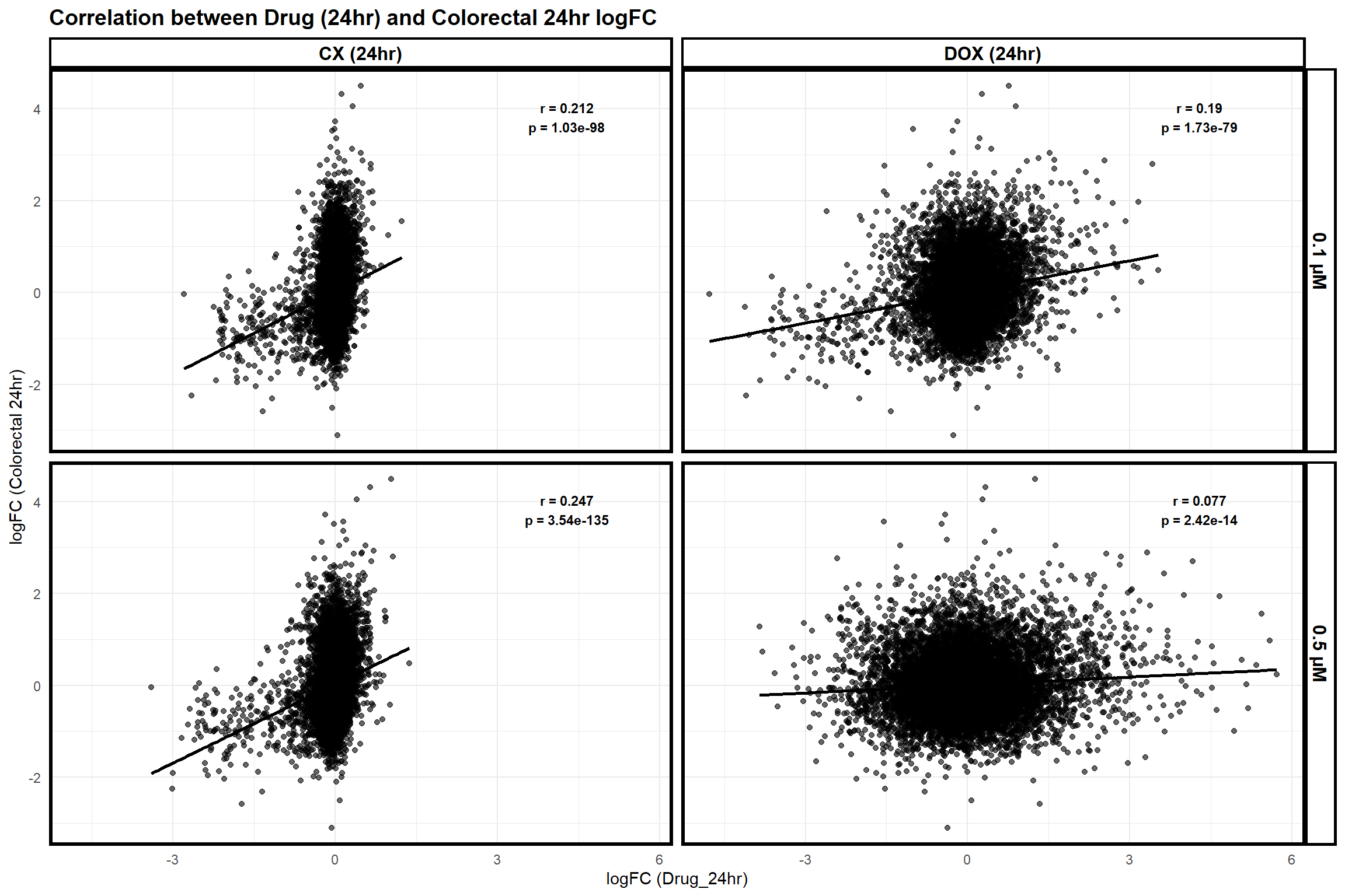

Past versions of Data_prep_24-1.png

Version	Author	Date
0649bff	sayanpaul01	2025-03-30
5b6c285	sayanpaul01	2025-02-28

📌 72hr

# Import the CSV file
data_72hr_logFC <- read.csv("data/Colorectal/72hrlogFC.csv", stringsAsFactors = FALSE)

# Map gene symbols to Entrez IDs using org.Hs.eg.db
data_72hr_logFC <- data_72hr_logFC %>%
  mutate(Entrez_ID = mapIds(org.Hs.eg.db,
                            keys = Symbol,
                            column = "ENTREZID",
                            keytype = "SYMBOL",
                            multiVals = "first"))

# Merge datasets on Entrez_ID for CX and DOX at both concentrations (48 hours)
merged_CX_0.1_48 <- merge(data_72hr_logFC, CX_0.1_48, by = "Entrez_ID")
merged_CX_0.5_48 <- merge(data_72hr_logFC, CX_0.5_48, by = "Entrez_ID")
merged_DOX_0.1_48 <- merge(data_72hr_logFC, DOX_0.1_48, by = "Entrez_ID")
merged_DOX_0.5_48 <- merge(data_72hr_logFC, DOX_0.5_48, by = "Entrez_ID")

# Remove NA values
merged_CX_0.1_48 <- na.omit(merged_CX_0.1_48)
merged_CX_0.5_48 <- na.omit(merged_CX_0.5_48)
merged_DOX_0.1_48 <- na.omit(merged_DOX_0.1_48)
merged_DOX_0.5_48 <- na.omit(merged_DOX_0.5_48)

# Rename columns explicitly to avoid conflicts
colnames(merged_CX_0.1_48) <- colnames(merged_CX_0.5_48) <-
  colnames(merged_DOX_0.1_48) <- colnames(merged_DOX_0.5_48) <-
  c("Entrez_ID", "Symbol_72hr", "logFC_72hr", "logFC_Drug", "AveExpr_Drug", "t_Drug", "P.Value_Drug", "adj.P.Val_Drug", "B_Drug")

# Add drug and concentration labels for faceting
merged_CX_0.1_48$Drug <- "CX (48hr)"
merged_CX_0.5_48$Drug <- "CX (48hr)"
merged_DOX_0.1_48$Drug <- "DOX (48hr)"
merged_DOX_0.5_48$Drug <- "DOX (48hr)"

merged_CX_0.1_48$Concentration <- "0.1 µM"
merged_CX_0.5_48$Concentration <- "0.5 µM"
merged_DOX_0.1_48$Concentration <- "0.1 µM"
merged_DOX_0.5_48$Concentration <- "0.5 µM"

# Combine all datasets into a single data frame
merged_data_48hr <- rbind(
  merged_CX_0.1_48[, c("Entrez_ID", "logFC_Drug", "logFC_72hr", "Concentration", "Drug")],
  merged_CX_0.5_48[, c("Entrez_ID", "logFC_Drug", "logFC_72hr", "Concentration", "Drug")],
  merged_DOX_0.1_48[, c("Entrez_ID", "logFC_Drug", "logFC_72hr", "Concentration", "Drug")],
  merged_DOX_0.5_48[, c("Entrez_ID", "logFC_Drug", "logFC_72hr", "Concentration", "Drug")]
)

# Calculate correlations for each facet
cor_CX_0.1_48 <- cor.test(merged_CX_0.1_48$logFC_Drug, merged_CX_0.1_48$logFC_72hr, method = "pearson")
cor_CX_0.5_48 <- cor.test(merged_CX_0.5_48$logFC_Drug, merged_CX_0.5_48$logFC_72hr, method = "pearson")
cor_DOX_0.1_48 <- cor.test(merged_DOX_0.1_48$logFC_Drug, merged_DOX_0.1_48$logFC_72hr, method = "pearson")
cor_DOX_0.5_48 <- cor.test(merged_DOX_0.5_48$logFC_Drug, merged_DOX_0.5_48$logFC_72hr, method = "pearson")

# Data frame for r and p-values annotations
correlation_data_48hr <- data.frame(
  Drug = rep(c("CX (48hr)", "DOX (48hr)"), each = 2),
  Concentration = rep(c("0.1 µM", "0.5 µM"), times = 2),
  x = max(merged_data_48hr$logFC_Drug, na.rm = TRUE) * 0.75,  # Adjusted placement for better fit
  y = max(merged_data_48hr$logFC_72hr, na.rm = TRUE) * 0.85,
  label = c(
    paste0("r = ", round(cor_CX_0.1_48$estimate, 3), "\np = ", signif(cor_CX_0.1_48$p.value, 3)),
    paste0("r = ", round(cor_CX_0.5_48$estimate, 3), "\np = ", signif(cor_CX_0.5_48$p.value, 3)),
    paste0("r = ", round(cor_DOX_0.1_48$estimate, 3), "\np = ", signif(cor_DOX_0.1_48$p.value, 3)),
    paste0("r = ", round(cor_DOX_0.5_48$estimate, 3), "\np = ", signif(cor_DOX_0.5_48$p.value, 3))
  )
)

# Create scatter plot with facets for concentration (vertically) and drug (horizontally)
scatter_plot_48hr <- ggplot(merged_data_48hr, aes(x = logFC_Drug, y = logFC_72hr)) +
  geom_point(alpha = 0.6, color = "black") +  # Black scatter points
  geom_smooth(method = "lm", color = "black", se = FALSE) +  # Black regression line
  labs(
    title = "Correlation between Drug (48hr) and Colorectal 72hr logFC",
    x = "logFC (Drug_48hr)",
    y = "logFC (Colorectal 72hr)"
  ) +
  theme_minimal() +
  theme(
    plot.title = element_text(size = 14, face = "bold"),

    # Outer box around the entire facet plot
    panel.border = element_rect(color = "black", fill = NA, linewidth = 2),

    # Black box around each facet title
    strip.background = element_rect(fill = "white", color = "black", linewidth = 1.5),
    strip.text = element_text(size = 12, face = "bold", color = "black")
  ) +

  # Facet by drug (horizontally) and concentration (vertically)
  facet_grid(Concentration ~ Drug) +

  # Add r and p-value in the upper-right corner of each facet with better fitting font size
  geom_text(data = correlation_data_48hr,
            aes(x = x, y = y, label = label),
            inherit.aes = FALSE, size = 3, fontface = "bold")  # Reduced font size for better fit

# Display plot
print(scatter_plot_48hr)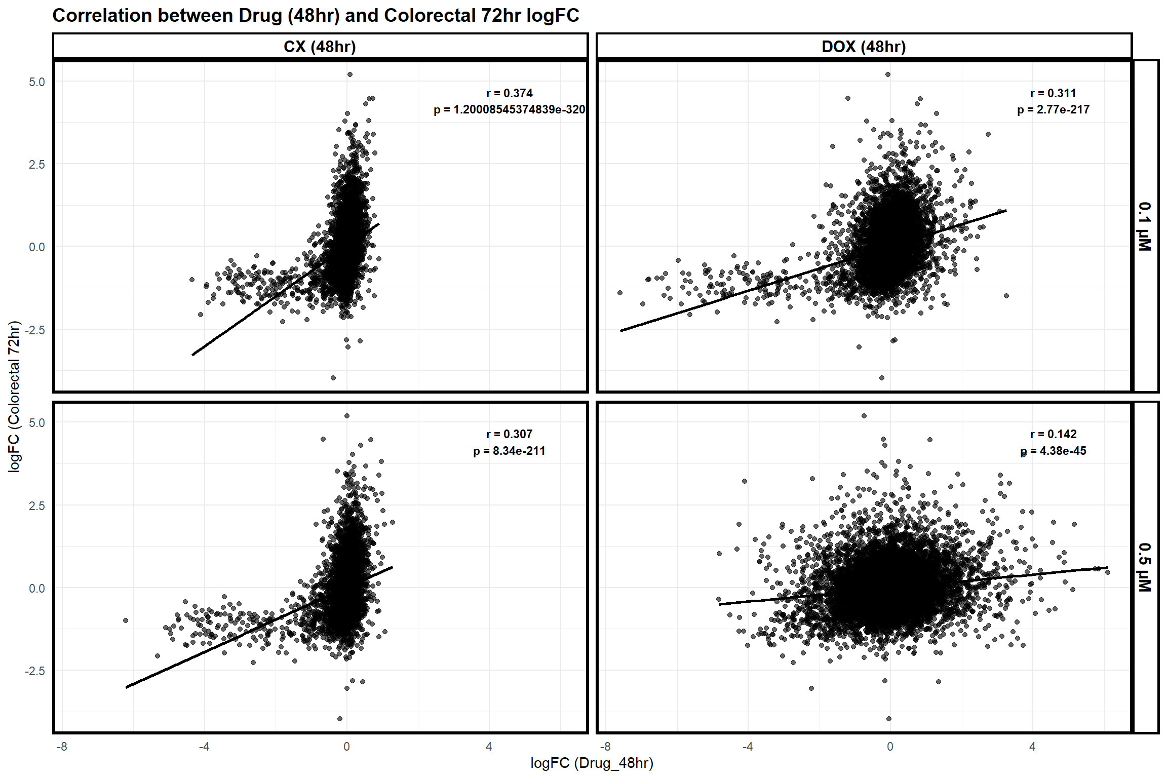

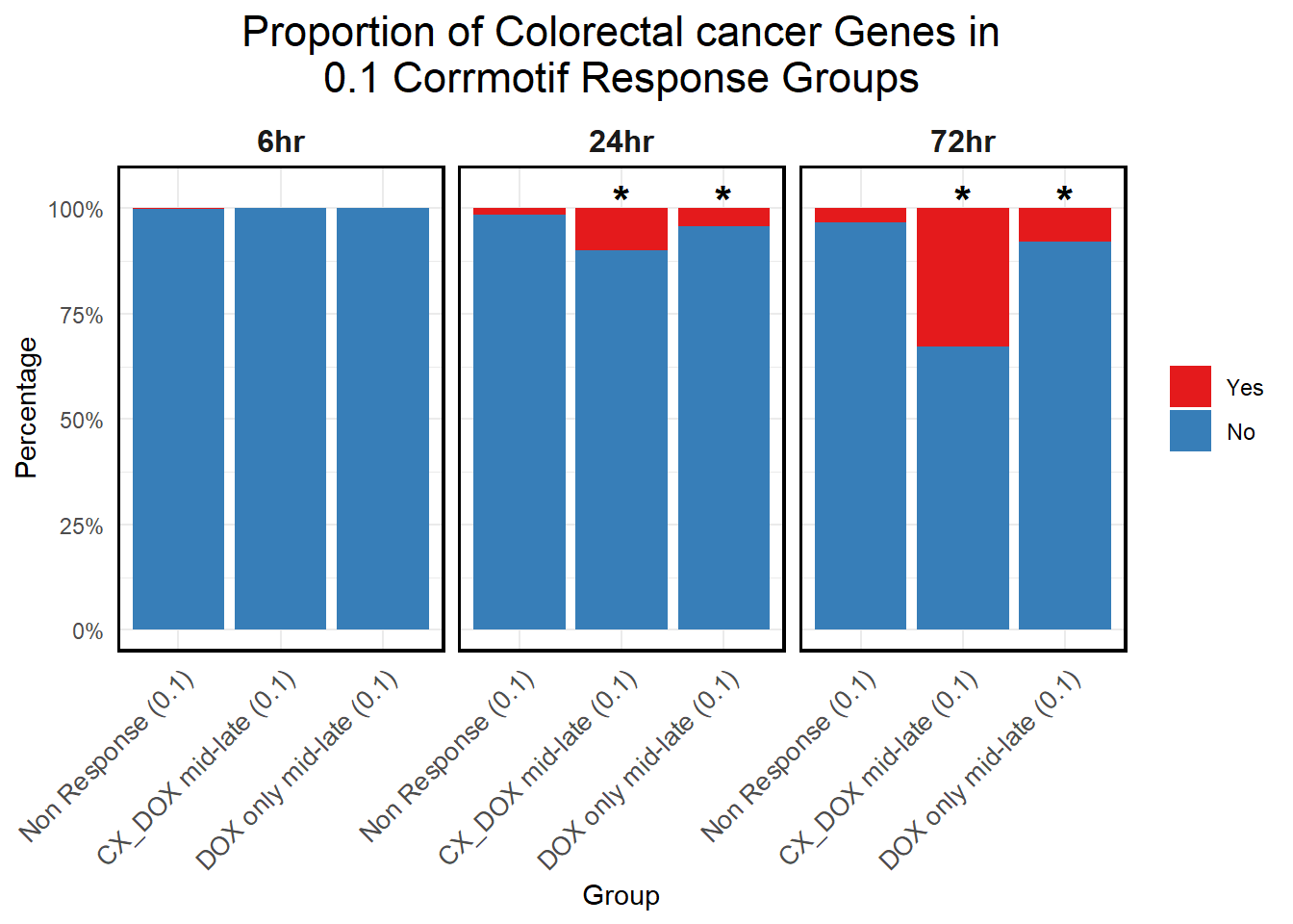
Past versions of Data_prep_72-1.png

Version	Author	Date
0649bff	sayanpaul01	2025-03-30
5b6c285	sayanpaul01	2025-02-28

📌 Proportion of Colorectal cancer Genes in corrmotif 0.1 micromolar

# Load necessary libraries
library(dplyr)
library(ggplot2)
library(tidyr)
library(org.Hs.eg.db)

# Load Colorectal Cancer Gene Lists
data_6hr <- read.csv("data/Colorectal/6hr.csv", stringsAsFactors = FALSE)
data_24hr <- read.csv("data/Colorectal/24hr.csv", stringsAsFactors = FALSE)
data_72hr <- read.csv("data/Colorectal/72hr.csv", stringsAsFactors = FALSE)

# Convert Gene Symbols to Entrez IDs
data_list <- list("6hr" = data_6hr, "24hr" = data_24hr, "72hr" = data_72hr)
data_list <- lapply(data_list, function(df) {
  df %>% mutate(Entrez_ID = mapIds(org.Hs.eg.db, keys = Symbol, column = "ENTREZID", keytype = "SYMBOL", multiVals = "first")) %>% na.omit()
})

lit_genes <- lapply(data_list, function(df) df$Entrez_ID)

# Load Corrmotif Groups for 0.1 Concentration
prob_groups_0.1 <- list(
  "Non Response (0.1)" = read.csv("data/prob_1_0.1.csv")$Entrez_ID,
  "CX_DOX mid-late (0.1)" = read.csv("data/prob_2_0.1.csv")$Entrez_ID,
  "DOX only mid-late (0.1)"= read.csv("data/prob_3_0.1.csv")$Entrez_ID
)

# Function to calculate proportions in colorectal cancer dataset
calculate_proportion <- function(deg_list, group_name, cancer_genes, timepoint) {
  total_group_genes <- length(deg_list)
  matched_genes <- sum(deg_list %in% cancer_genes)
  
  data.frame(
    Group = group_name,
    Timepoint = timepoint,
    Colorectal_DEGs = matched_genes,
    Non_Colorectal_DEGs = total_group_genes - matched_genes
  ) %>%
    mutate(
      Yes_Proportion = (Colorectal_DEGs / total_group_genes) * 100,
      No_Proportion = (Non_Colorectal_DEGs / total_group_genes) * 100
    )
}

# Calculate Proportions for Each Timepoint
proportion_data <- bind_rows(
  lapply(names(lit_genes), function(tp) calculate_proportion(prob_groups_0.1[["Non Response (0.1)"]], "Non Response (0.1)", lit_genes[[tp]], tp)),
  lapply(names(lit_genes), function(tp) calculate_proportion(prob_groups_0.1[["CX_DOX mid-late (0.1)"]], "CX_DOX mid-late (0.1)", lit_genes[[tp]], tp)),
  lapply(names(lit_genes), function(tp) calculate_proportion(prob_groups_0.1[["DOX only mid-late (0.1)"]], "DOX only mid-late (0.1)", lit_genes[[tp]], tp)))
  
  

# Convert Data to Long Format for Faceting
proportion_long <- proportion_data %>%
  pivot_longer(cols = c(Yes_Proportion, No_Proportion), names_to = "Category", values_to = "Percentage") %>%
  mutate(Category = ifelse(Category == "Yes_Proportion", "Yes", "No"))

# Perform Chi-Square Test Comparing Groups to Non-Response
test_results <- data.frame(Group = character(), Timepoint = character(), P_Value = numeric())

target_groups <- c("CX_DOX mid-late (0.1)", "DOX only mid-late (0.1)")
for (tp in names(lit_genes)) {
  for (grp in target_groups) {
    contingency_table <- matrix(
      c(
        sum(prob_groups_0.1[[grp]] %in% lit_genes[[tp]]),
        length(prob_groups_0.1[[grp]]) - sum(prob_groups_0.1[[grp]] %in% lit_genes[[tp]]),
        sum(prob_groups_0.1[["Non Response (0.1)"]] %in% lit_genes[[tp]]),
        length(prob_groups_0.1[["Non Response (0.1)"]]) - sum(prob_groups_0.1[["Non Response (0.1)"]] %in% lit_genes[[tp]])
      ),
      nrow = 2, byrow = TRUE
    )
    test_result <- chisq.test(contingency_table)
    test_results <- rbind(test_results, data.frame(Group = grp, Timepoint = tp, P_Value = test_result$p.value))
  }
}

Warning in chisq.test(contingency_table): Chi-squared approximation may be
incorrect
Warning in chisq.test(contingency_table): Chi-squared approximation may be
incorrect

# Add Significance Stars
test_results$Significant <- ifelse(test_results$P_Value < 0.05, "*", "")
proportion_long <- left_join(proportion_long, test_results, by = c("Group", "Timepoint"))

# Ensure Correct Ordering
proportion_long$Group <- factor(proportion_long$Group, levels = c("Non Response (0.1)", "CX_DOX mid-late (0.1)", "DOX only mid-late (0.1)"))
proportion_long$Timepoint <- factor(proportion_long$Timepoint, levels = c("6hr", "24hr", "72hr"))
proportion_long$Category <- factor(proportion_long$Category, levels = c("Yes", "No"))

# Generate Stacked Bar Plot with Faceting and Significance Annotations
ggplot(proportion_long, aes(x = Group, y = Percentage, fill = Category)) +
  geom_bar(stat = "identity", position = "stack") +
  facet_wrap(~Timepoint, scales = "fixed") +
  geom_text(data = subset(proportion_long, Significant == "*"),
            aes(x = Group, y = 102, label = "*"),
            size = 6, color = "black", fontface = "bold") +
  scale_y_continuous(labels = scales::percent_format(scale = 1), limits = c(0, 105)) +
  scale_fill_manual(values = c("Yes" = "#e41a1c", "No" = "#377eb8")) +
  labs(
    title = "Proportion of Colorectal cancer Genes in\n0.1 Corrmotif Response Groups",
    x = "Group",
    y = "Percentage",
    fill = "Category"
  ) +
  theme_minimal() +
  theme(
    plot.title = element_text(size = rel(1.5), hjust = 0.5),
    axis.text.x = element_text(size = 10, angle = 45, hjust = 1),
    legend.title = element_blank(),
    panel.border = element_rect(color = "black", fill = NA, linewidth = 1.2),
    strip.background = element_blank(),
    strip.text = element_text(size = 12, face = "bold")
  )

Past versions of "prop DNA-1.png"

Version	Author	Date
0649bff	sayanpaul01	2025-03-30
0aec578	sayanpaul01	2025-03-06
1c452e8	sayanpaul01	2025-03-05

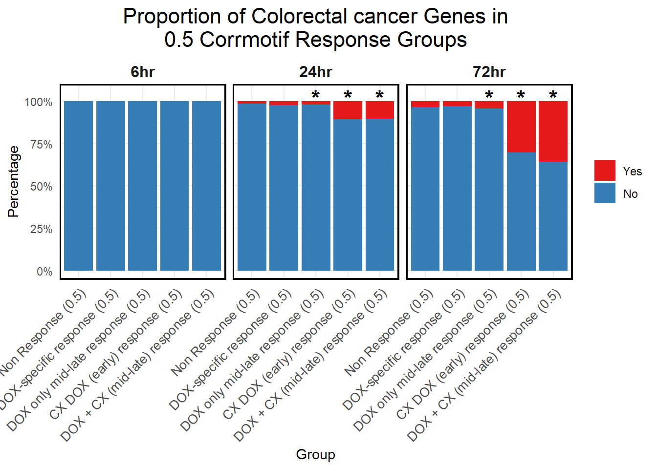
📌 Proportion of Colorectal cancer Genes in corrmotif 0.5 micromolar

# Load necessary libraries
library(dplyr)
library(ggplot2)
library(tidyr)
library(org.Hs.eg.db)

# Load Colorectal Cancer Gene Lists
data_6hr <- read.csv("data/Colorectal/6hr.csv", stringsAsFactors = FALSE)
data_24hr <- read.csv("data/Colorectal/24hr.csv", stringsAsFactors = FALSE)
data_72hr <- read.csv("data/Colorectal/72hr.csv", stringsAsFactors = FALSE)

# Convert Gene Symbols to Entrez IDs
data_list <- list("6hr" = data_6hr, "24hr" = data_24hr, "72hr" = data_72hr)
data_list <- lapply(data_list, function(df) {
  df %>% mutate(Entrez_ID = mapIds(org.Hs.eg.db, keys = Symbol, column = "ENTREZID", keytype = "SYMBOL", multiVals = "first")) %>% na.omit()
})

lit_genes <- lapply(data_list, function(df) df$Entrez_ID)

# Load Corrmotif Groups for 0.5 Concentration
prob_groups_0.5 <- list(
  "Non Response (0.5)" = read.csv("data/prob_1_0.5.csv")$Entrez_ID,
  "DOX-specific response (0.5)" = read.csv("data/prob_2_0.5.csv")$Entrez_ID,
  "DOX only mid-late response (0.5)" = read.csv("data/prob_3_0.5.csv")$Entrez_ID,
  "CX DOX (early) response (0.5)" = read.csv("data/prob_4_0.5.csv")$Entrez_ID,
  "DOX + CX (mid-late) response (0.5)" = read.csv("data/prob_5_0.5.csv")$Entrez_ID
)

# Function to calculate proportions in colorectal cancer dataset
calculate_proportion <- function(deg_list, group_name, cancer_genes, timepoint) {
  total_group_genes <- length(deg_list)
  matched_genes <- sum(deg_list %in% cancer_genes)
  
  data.frame(
    Group = group_name,
    Timepoint = timepoint,
    Colorectal_DEGs = matched_genes,
    Non_Colorectal_DEGs = total_group_genes - matched_genes
  ) %>%
    mutate(
      Yes_Proportion = (Colorectal_DEGs / total_group_genes) * 100,
      No_Proportion = (Non_Colorectal_DEGs / total_group_genes) * 100
    )
}

# Calculate Proportions for Each Timepoint
proportion_data <- bind_rows(
  lapply(names(lit_genes), function(tp) calculate_proportion(prob_groups_0.5[["Non Response (0.5)"]], "Non Response (0.5)", lit_genes[[tp]], tp)),
  lapply(names(lit_genes), function(tp) calculate_proportion(prob_groups_0.5[["DOX-specific response (0.5)"]], "DOX-specific response (0.5)", lit_genes[[tp]], tp)),
  lapply(names(lit_genes), function(tp) calculate_proportion(prob_groups_0.5[["DOX only mid-late response (0.5)"]], "DOX only mid-late response (0.5)", lit_genes[[tp]], tp)),
  lapply(names(lit_genes), function(tp) calculate_proportion(prob_groups_0.5[["CX DOX (early) response (0.5)"]], "CX DOX (early) response (0.5)", lit_genes[[tp]], tp)),
  lapply(names(lit_genes), function(tp) calculate_proportion(prob_groups_0.5[["DOX + CX (mid-late) response (0.5)"]], "DOX + CX (mid-late) response (0.5)", lit_genes[[tp]], tp))
)

# Convert Data to Long Format for Faceting
proportion_long <- proportion_data %>%
  pivot_longer(cols = c(Yes_Proportion, No_Proportion), names_to = "Category", values_to = "Percentage") %>%
  mutate(Category = ifelse(Category == "Yes_Proportion", "Yes", "No"))

# Perform Chi-Square Test Comparing Groups to Non-Response
test_results <- data.frame(Group = character(), Timepoint = character(), P_Value = numeric())

target_groups <- c("DOX-specific response (0.5)", "DOX only mid-late response (0.5)", "CX DOX (early) response (0.5)", "DOX + CX (mid-late) response (0.5)")
for (tp in names(lit_genes)) {
  for (grp in target_groups) {
    contingency_table <- matrix(
      c(
        sum(prob_groups_0.5[[grp]] %in% lit_genes[[tp]]),
        length(prob_groups_0.5[[grp]]) - sum(prob_groups_0.5[[grp]] %in% lit_genes[[tp]]),
        sum(prob_groups_0.5[["Non Response (0.5)"]] %in% lit_genes[[tp]]),
        length(prob_groups_0.5[["Non Response (0.5)"]]) - sum(prob_groups_0.5[["Non Response (0.5)"]] %in% lit_genes[[tp]])
      ),
      nrow = 2, byrow = TRUE
    )
    test_result <- chisq.test(contingency_table)
    test_results <- rbind(test_results, data.frame(Group = grp, Timepoint = tp, P_Value = test_result$p.value))
  }
}

Warning in chisq.test(contingency_table): Chi-squared approximation may be
incorrect
Warning in chisq.test(contingency_table): Chi-squared approximation may be
incorrect
Warning in chisq.test(contingency_table): Chi-squared approximation may be
incorrect
Warning in chisq.test(contingency_table): Chi-squared approximation may be
incorrect
Warning in chisq.test(contingency_table): Chi-squared approximation may be
incorrect
Warning in chisq.test(contingency_table): Chi-squared approximation may be
incorrect
Warning in chisq.test(contingency_table): Chi-squared approximation may be
incorrect

# Add Significance Stars
test_results$Significant <- ifelse(test_results$P_Value < 0.05, "*", "")
proportion_long <- left_join(proportion_long, test_results, by = c("Group", "Timepoint"))

# Ensure Correct Ordering
proportion_long$Group <- factor(proportion_long$Group, levels = c("Non Response (0.5)", "DOX-specific response (0.5)", "DOX only mid-late response (0.5)", "CX DOX (early) response (0.5)", "DOX + CX (mid-late) response (0.5)"))
proportion_long$Timepoint <- factor(proportion_long$Timepoint, levels = c("6hr", "24hr", "72hr"))
proportion_long$Category <- factor(proportion_long$Category, levels = c("Yes", "No"))

# Generate Stacked Bar Plot with Faceting and Significance Annotations
ggplot(proportion_long, aes(x = Group, y = Percentage, fill = Category)) +
  geom_bar(stat = "identity", position = "stack") +
  facet_wrap(~Timepoint, scales = "fixed") +
  geom_text(data = subset(proportion_long, Significant == "*"),
            aes(x = Group, y = 102, label = "*"),
            size = 6, color = "black", fontface = "bold") +
  scale_y_continuous(labels = scales::percent_format(scale = 1), limits = c(0, 105)) +
  scale_fill_manual(values = c("Yes" = "#e41a1c", "No" = "#377eb8")) +
  labs(
    title = "Proportion of Colorectal cancer Genes in\n0.5 Corrmotif Response Groups",
    x = "Group",
    y = "Percentage",
    fill = "Category"
  ) +
  theme_minimal() +
  theme(
    plot.title = element_text(size = rel(1.5), hjust = 0.5),
    axis.text.x = element_text(size = 10, angle = 45, hjust = 1),
    legend.title = element_blank(),
    panel.border = element_rect(color = "black", fill = NA, linewidth = 1.2),
    strip.background = element_blank(),
    strip.text = element_text(size = 12, face = "bold")
  )

Past versions of "prop 0.5-1.png"

Version	Author	Date
0649bff	sayanpaul01	2025-03-30
1c452e8	sayanpaul01	2025-03-05

📌 Correlation heatmap

# Load necessary libraries
library(ggplot2)
library(reshape2)
library(dplyr)
library(org.Hs.eg.db)
library(biomaRt)

# Load colorectal cancer logFC data for 6hr, 24hr, and 72hr
data_6hr_logFC <- read.csv("data/Colorectal/6hrlogFC.csv", stringsAsFactors = FALSE)
data_24hr_logFC <- read.csv("data/Colorectal/24hrlogFC.csv", stringsAsFactors = FALSE)
data_72hr_logFC <- read.csv("data/Colorectal/72hrlogFC.csv", stringsAsFactors = FALSE)

# Map gene symbols to Entrez IDs
map_entrez <- function(data) {
  data %>%
    mutate(Entrez_ID = mapIds(org.Hs.eg.db,
                              keys = Symbol,
                              column = "ENTREZID",
                              keytype = "SYMBOL",
                              multiVals = "first"))
}

data_6hr_logFC <- map_entrez(data_6hr_logFC)
data_24hr_logFC <- map_entrez(data_24hr_logFC)
data_72hr_logFC <- map_entrez(data_72hr_logFC)

# Load CX-5461 and DOX logFC data for 3hr, 24hr, 48hr
CX_0.1_3 <- read.csv("data/DEGs/Toptable_CX_0.1_3.csv", stringsAsFactors = FALSE)
CX_0.5_3 <- read.csv("data/DEGs/Toptable_CX_0.5_3.csv", stringsAsFactors = FALSE)
CX_0.1_24 <- read.csv("data/DEGs/Toptable_CX_0.1_24.csv", stringsAsFactors = FALSE)
CX_0.5_24 <- read.csv("data/DEGs/Toptable_CX_0.5_24.csv", stringsAsFactors = FALSE)
CX_0.1_48 <- read.csv("data/DEGs/Toptable_CX_0.1_48.csv", stringsAsFactors = FALSE)
CX_0.5_48 <- read.csv("data/DEGs/Toptable_CX_0.5_48.csv", stringsAsFactors = FALSE)

DOX_0.1_3 <- read.csv("data/DEGs/Toptable_DOX_0.1_3.csv", stringsAsFactors = FALSE)
DOX_0.5_3 <- read.csv("data/DEGs/Toptable_DOX_0.5_3.csv", stringsAsFactors = FALSE)
DOX_0.1_24 <- read.csv("data/DEGs/Toptable_DOX_0.1_24.csv", stringsAsFactors = FALSE)
DOX_0.5_24 <- read.csv("data/DEGs/Toptable_DOX_0.5_24.csv", stringsAsFactors = FALSE)
DOX_0.1_48 <- read.csv("data/DEGs/Toptable_DOX_0.1_48.csv", stringsAsFactors = FALSE)
DOX_0.5_48 <- read.csv("data/DEGs/Toptable_DOX_0.5_48.csv", stringsAsFactors = FALSE)

# Function to merge colorectal and drug datasets
merge_data <- function(colorectal_data, drug_data) {
  merged <- merge(colorectal_data, drug_data, by = "Entrez_ID")
  na.omit(merged)  # Remove NA values
}

# Merge data for all timepoints and concentrations
merged_CX_0.1_3 <- merge_data(data_6hr_logFC, CX_0.1_3)
merged_CX_0.5_3 <- merge_data(data_6hr_logFC, CX_0.5_3)
merged_DOX_0.1_3 <- merge_data(data_6hr_logFC, DOX_0.1_3)
merged_DOX_0.5_3 <- merge_data(data_6hr_logFC, DOX_0.5_3)

merged_CX_0.1_24 <- merge_data(data_24hr_logFC, CX_0.1_24)
merged_CX_0.5_24 <- merge_data(data_24hr_logFC, CX_0.5_24)
merged_DOX_0.1_24 <- merge_data(data_24hr_logFC, DOX_0.1_24)
merged_DOX_0.5_24 <- merge_data(data_24hr_logFC, DOX_0.5_24)

merged_CX_0.1_48 <- merge_data(data_72hr_logFC, CX_0.1_48)
merged_CX_0.5_48 <- merge_data(data_72hr_logFC, CX_0.5_48)
merged_DOX_0.1_48 <- merge_data(data_72hr_logFC, DOX_0.1_48)
merged_DOX_0.5_48 <- merge_data(data_72hr_logFC, DOX_0.5_48)

# Compute correlation coefficients (Pearson)
compute_correlation <- function(df) {
  cor.test(df$logFC.x, df$logFC.y, method = "pearson")$estimate
}

cor_CX_0.1_3 <- compute_correlation(merged_CX_0.1_3)
cor_CX_0.5_3 <- compute_correlation(merged_CX_0.5_3)
cor_DOX_0.1_3 <- compute_correlation(merged_DOX_0.1_3)
cor_DOX_0.5_3 <- compute_correlation(merged_DOX_0.5_3)

cor_CX_0.1_24 <- compute_correlation(merged_CX_0.1_24)
cor_CX_0.5_24 <- compute_correlation(merged_CX_0.5_24)
cor_DOX_0.1_24 <- compute_correlation(merged_DOX_0.1_24)
cor_DOX_0.5_24 <- compute_correlation(merged_DOX_0.5_24)

cor_CX_0.1_48 <- compute_correlation(merged_CX_0.1_48)
cor_CX_0.5_48 <- compute_correlation(merged_CX_0.5_48)
cor_DOX_0.1_48 <- compute_correlation(merged_DOX_0.1_48)
cor_DOX_0.5_48 <- compute_correlation(merged_DOX_0.5_48)

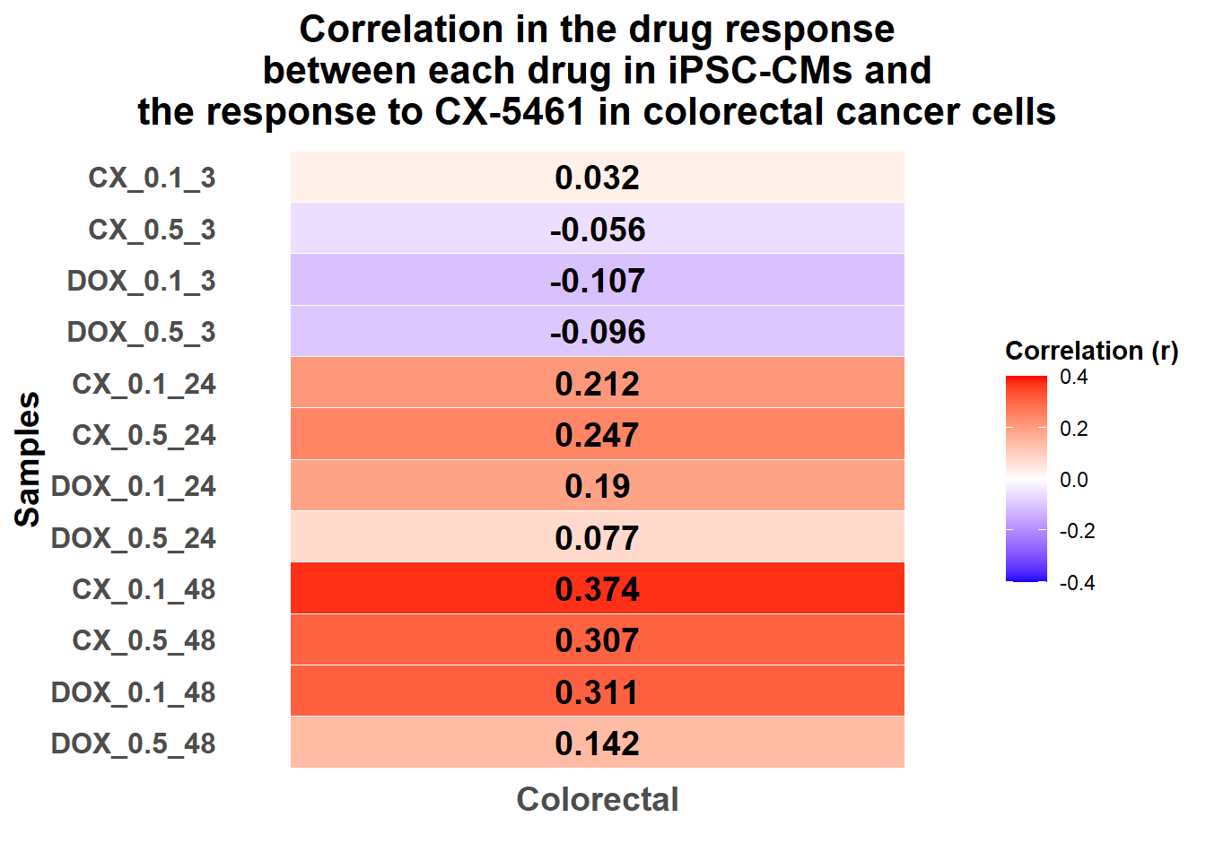
# Define correlation values from previously computed Pearson correlations
correlation_data <- data.frame(
  Sample = c("CX_0.1_3", "CX_0.5_3", "DOX_0.1_3", "DOX_0.5_3",
             "CX_0.1_24", "CX_0.5_24", "DOX_0.1_24", "DOX_0.5_24",
             "CX_0.1_48", "CX_0.5_48", "DOX_0.1_48", "DOX_0.5_48"),
  Correlation = c(
    cor_CX_0.1_3, cor_CX_0.5_3, cor_DOX_0.1_3, cor_DOX_0.5_3,
    cor_CX_0.1_24, cor_CX_0.5_24, cor_DOX_0.1_24, cor_DOX_0.5_24,
    cor_CX_0.1_48, cor_CX_0.5_48, cor_DOX_0.1_48, cor_DOX_0.5_48
  )
)

# Add a single column category for labeling
correlation_data$Comparison <- "Colorectal"

# Convert to long format for ggplot
heatmap_data_long <- melt(correlation_data, id.vars = c("Sample", "Comparison"))

# Ensure the Y-axis follows the correct top-down ordering
heatmap_data_long$Sample <- factor(heatmap_data_long$Sample, levels = rev(c(  # Reversed order
  "CX_0.1_3", "CX_0.5_3", "DOX_0.1_3", "DOX_0.5_3",
  "CX_0.1_24", "CX_0.5_24", "DOX_0.1_24", "DOX_0.5_24",
  "CX_0.1_48", "CX_0.5_48", "DOX_0.1_48", "DOX_0.5_48"
)))

# Create the correctly ordered single-column heatmap
ggplot(heatmap_data_long, aes(x = Comparison, y = Sample, fill = value)) +
  geom_tile(color = "white") +
  scale_fill_gradient2(
    low = "blue", mid = "white", high = "red", limits = c(-0.4,0.4)) +  # Updated scale
  geom_text(aes(label = round(value, 3)), color = "black", size = 5, fontface = "bold") +
  labs(
    x = "", y = "Samples", fill = "Correlation (r)",
    title = "Correlation in the drug response\nbetween each drug in iPSC-CMs and\nthe response to CX-5461 in colorectal cancer cells"
  ) +
  theme_minimal() +
  theme(
    axis.text.x = element_text(face = "bold", size = 14),
    axis.text.y = element_text(face = "bold", size = 12),
    axis.title.y = element_text(face = "bold", size = 14),
    plot.title = element_text(face = "bold", hjust = 0.5, size = 16),
    legend.title = element_text(face = "bold"),
    panel.grid = element_blank()
  )

Past versions of colr-1.png

Version	Author	Date
488c5c4	sayanpaul01	2025-06-02
bf87a05	sayanpaul01	2025-03-30
0649bff	sayanpaul01	2025-03-30
44d47e5	sayanpaul01	2025-03-16

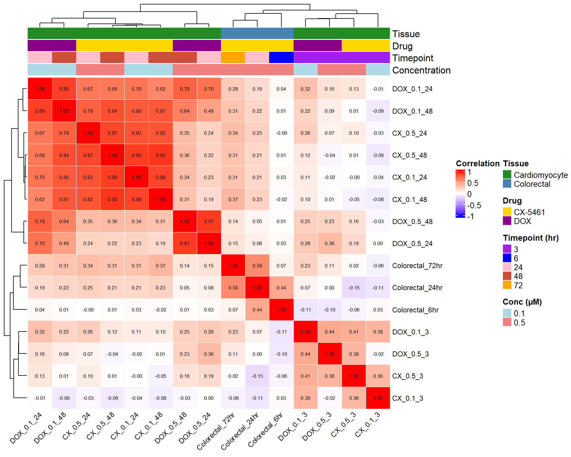
📌 logFC Correlation heatmap (Complete dataset)

# 📦 Load Required Libraries
library(data.table)

Warning: package 'data.table' was built under R version 4.3.3

library(tidyverse)
library(janitor)

Warning: package 'janitor' was built under R version 4.3.3

library(org.Hs.eg.db)
library(AnnotationDbi)
library(ComplexHeatmap)

Warning: package 'ComplexHeatmap' was built under R version 4.3.1

library(circlize)

Warning: package 'circlize' was built under R version 4.3.3

library(RColorBrewer)
library(grid)

# 🧠 Function to map gene SYMBOL to Entrez ID for colorectal datasets
map_entrez <- function(df) {
  df %>%
    mutate(entrez_id = mapIds(
      org.Hs.eg.db,
      keys = Symbol,
      column = "ENTREZID",
      keytype = "SYMBOL",
      multiVals = "first"
    )) %>%
    mutate(entrez_id = as.character(entrez_id))
}

# 📁 Define All logFC Input Files (CX-5461, DOX, Colorectal)
logfc_files <- list(
  "CX_0.1_3"   = "data/DEGs/Toptable_CX_0.1_3.csv",
  "CX_0.1_24"  = "data/DEGs/Toptable_CX_0.1_24.csv",
  "CX_0.1_48"  = "data/DEGs/Toptable_CX_0.1_48.csv",
  "CX_0.5_3"   = "data/DEGs/Toptable_CX_0.5_3.csv",
  "CX_0.5_24"  = "data/DEGs/Toptable_CX_0.5_24.csv",
  "CX_0.5_48"  = "data/DEGs/Toptable_CX_0.5_48.csv",
  "DOX_0.1_3"  = "data/DEGs/Toptable_DOX_0.1_3.csv",
  "DOX_0.1_24" = "data/DEGs/Toptable_DOX_0.1_24.csv",
  "DOX_0.1_48" = "data/DEGs/Toptable_DOX_0.1_48.csv",
  "DOX_0.5_3"  = "data/DEGs/Toptable_DOX_0.5_3.csv",
  "DOX_0.5_24" = "data/DEGs/Toptable_DOX_0.5_24.csv",
  "DOX_0.5_48" = "data/DEGs/Toptable_DOX_0.5_48.csv",
  "Colorectal_6hr"  = "data/Colorectal/6hrlogFC.csv",
  "Colorectal_24hr" = "data/Colorectal/24hrlogFC.csv",
  "Colorectal_72hr" = "data/Colorectal/72hrlogFC.csv"
)

# 🔁 Process All Files: Extract clean (Entrez_ID, logFC) tibble per sample
logfc_list <- map2(names(logfc_files), logfc_files, function(name, path) {
  df <- fread(path, data.table = FALSE) %>% as_tibble()

  # Map Entrez ID for colorectal
  if (grepl("colorectal", tolower(name))) {
    df <- map_entrez(df)
  }

  # Auto-detect columns
  logfc_col <- names(df)[str_detect(names(df), regex("^logfc$", ignore_case = TRUE))][1]
  entrez_col <- names(df)[str_detect(names(df), regex("entrez.*id", ignore_case = TRUE))][1]

  if (is.na(logfc_col) || is.na(entrez_col)) {
    stop(paste("Missing columns in:", name,
               "\nAvailable columns:", paste(names(df), collapse = ", ")))
  }

  df %>%
    filter(!is.na(.data[[logfc_col]]), !is.na(.data[[entrez_col]])) %>%
    mutate(entrez_id = as.character(.data[[entrez_col]])) %>%
    distinct(entrez_id, .keep_all = TRUE) %>%
    dplyr::select(entrez_id, logFC = all_of(logfc_col)) %>%
    dplyr::rename(!!name := logFC)
})




# 🧬 Identify Common Entrez_IDs Across All Datasets
common_ids <- purrr::reduce(logfc_list, inner_join, by = "entrez_id") %>%
  pull(entrez_id) %>%
  unique()


# 🧱 Build Final logFC Matrix (Entrez_ID × Sample)
logfc_matrix <- map(logfc_list, ~ filter(.x, entrez_id %in% common_ids)) %>%
  purrr::reduce(inner_join, by = "entrez_id") %>%
  column_to_rownames("entrez_id") %>%
  as.matrix()

# ✅ Assume logfc_matrix is already created
# Rows = Entrez_IDs, Columns = Samples
sample_names <- colnames(logfc_matrix)

# 📁 Create Metadata Inline
metadata <- tibble(Sample = sample_names) %>%
  mutate(
    Drug = case_when(
      str_detect(Sample, "CX") ~ "CX-5461",
      str_detect(Sample, "DOX") ~ "DOX",
      str_detect(Sample, "Colorectal") ~ "CX-5461"
    ),
    Tissue = case_when(
      str_detect(Sample, "Colorectal") ~ "Colorectal",
      TRUE ~ "Cardiomyocyte"
    ),
    Time = case_when(
      str_detect(Sample, "6hr") ~ "6",
      str_detect(Sample, "24") ~ "24",
      str_detect(Sample, "72") ~ "72",
      str_detect(Sample, "48") ~ "48",
      str_detect(Sample, "3") ~ "3",
      TRUE ~ NA_character_
    ),
    Conc = case_when(
      str_detect(Sample, "Colorectal") ~ "0.5",
      str_detect(Sample, "0.1") ~ "0.1",
      str_detect(Sample, "0.5") ~ "0.5",
      TRUE ~ NA_character_
    )
  )

metadata <- metadata %>%
  mutate(Time = factor(Time, levels = c("3", "6", "24", "48", "72")))

# 🎨 Define Annotation Colors
time_colors <- c("3" = "purple", "6" = "blue", "24" = "pink", "48" = "tomato3", "72" = "orange")
drug_colors <- c("CX-5461" = "gold", "DOX" = "magenta4")
conc_colors <- c("0.1" = "lightblue", "0.5" = "lightcoral")
tissue_colors <- c("Cardiomyocyte" = "forestgreen", "Colorectal" = "steelblue")

# 🔝 Top Annotation Track
top_annot <- HeatmapAnnotation(
  Tissue = metadata$Tissue,
  Drug = metadata$Drug,
  Timepoint = metadata$Time,
  Concentration = metadata$Conc,
  col = list(
    Tissue = tissue_colors,
    Drug = drug_colors,
    Timepoint = time_colors,
    Concentration = conc_colors
  ),
  annotation_legend_param = list(
    Tissue = list(title = "Tissue"),
    Drug = list(title = "Drug"),
    Timepoint = list(title = "Timepoint (hr)"),
    Concentration = list(title = "Conc (µM)")
  )
)

# 📊 Compute Pearson Correlation Matrix
pearson_matrix <- cor(logfc_matrix, method = "pearson")

# 🎨 Color Function for Pearson r
col_fun <- colorRamp2(c(-1, 0, 1), c("blue", "white", "red"))


# 🔥 Draw Pearson Correlation Heatmap
Heatmap(
  pearson_matrix,
  name = "Pearson\nCorrelation",
  col = col_fun,
  top_annotation = top_annot,
  cluster_rows = TRUE,
  cluster_columns = TRUE,
  row_names_gp = gpar(fontsize = 9),
  column_names_gp = gpar(fontsize = 9),
  column_names_rot = 45,
  rect_gp = gpar(col = "white", lwd = 0.5),
  cell_fun = function(j, i, x, y, w, h, fill) {
    grid.text(sprintf("%.2f", pearson_matrix[i, j]), x, y, gp = gpar(fontsize = 6.5))
  },
  heatmap_legend_param = list(
    title = "Correlation",
    at = c(-1, -0.5, 0, 0.5, 1),
    labels = c("-1", "-0.5", "0", "0.5", "1"),
    direction = "vertical"
  )
)

Past versions of colr2-1.png

Version	Author	Date
488c5c4	sayanpaul01	2025-06-02

Session information

sessionInfo()

R version 4.3.0 (2023-04-21 ucrt)
Platform: x86_64-w64-mingw32/x64 (64-bit)
Running under: Windows 11 x64 (build 26100)

Matrix products: default


locale:
[1] LC_COLLATE=English_United States.utf8 
[2] LC_CTYPE=English_United States.utf8   
[3] LC_MONETARY=English_United States.utf8
[4] LC_NUMERIC=C                          
[5] LC_TIME=English_United States.utf8    

time zone: America/Chicago
tzcode source: internal

attached base packages:
[1] grid      stats4    stats     graphics  grDevices utils     datasets 
[8] methods   base     

other attached packages:
 [1] RColorBrewer_1.1-3     circlize_0.4.16        ComplexHeatmap_2.18.0 
 [4] janitor_2.2.1          data.table_1.17.0      reshape2_1.4.4        
 [7] biomaRt_2.58.2         clusterProfiler_4.10.1 org.Hs.eg.db_3.18.0   
[10] AnnotationDbi_1.64.1   IRanges_2.36.0         S4Vectors_0.40.2      
[13] Biobase_2.62.0         BiocGenerics_0.48.1    lubridate_1.9.4       
[16] forcats_1.0.0          stringr_1.5.1          dplyr_1.1.4           
[19] purrr_1.0.4            readr_2.1.5            tidyr_1.3.1           
[22] tibble_3.2.1           ggplot2_3.5.2          tidyverse_2.0.0       

loaded via a namespace (and not attached):
  [1] shape_1.4.6.1           rstudioapi_0.17.1       jsonlite_2.0.0         
  [4] magrittr_2.0.3          magick_2.8.6            farver_2.1.2           
  [7] rmarkdown_2.29          GlobalOptions_0.1.2     fs_1.6.3               
 [10] zlibbioc_1.48.2         vctrs_0.6.5             Cairo_1.6-2            
 [13] memoise_2.0.1           RCurl_1.98-1.17         ggtree_3.10.1          
 [16] htmltools_0.5.8.1       progress_1.2.3          curl_6.2.2             
 [19] gridGraphics_0.5-1      sass_0.4.10             bslib_0.9.0            
 [22] plyr_1.8.9              cachem_1.1.0            whisker_0.4.1          
 [25] igraph_2.1.4            iterators_1.0.14        lifecycle_1.0.4        
 [28] pkgconfig_2.0.3         Matrix_1.6-1.1          R6_2.6.1               
 [31] fastmap_1.2.0           gson_0.1.0              clue_0.3-66            
 [34] snakecase_0.11.1        GenomeInfoDbData_1.2.11 digest_0.6.34          
 [37] aplot_0.2.5             enrichplot_1.22.0       colorspace_2.1-0       
 [40] patchwork_1.3.0         rprojroot_2.0.4         RSQLite_2.3.9          
 [43] filelock_1.0.3          labeling_0.4.3          timechange_0.3.0       
 [46] mgcv_1.9-3              httr_1.4.7              polyclip_1.10-7        
 [49] compiler_4.3.0          doParallel_1.0.17       bit64_4.6.0-1          
 [52] withr_3.0.2             BiocParallel_1.36.0     viridis_0.6.5          
 [55] DBI_1.2.3               ggforce_0.4.2           MASS_7.3-60            
 [58] rappdirs_0.3.3          rjson_0.2.23            HDO.db_0.99.1          
 [61] tools_4.3.0             ape_5.8-1               scatterpie_0.2.4       
 [64] httpuv_1.6.15           glue_1.7.0              nlme_3.1-168           
 [67] GOSemSim_2.28.1         promises_1.3.2          shadowtext_0.1.4       
 [70] cluster_2.1.8.1         fgsea_1.28.0            generics_0.1.3         
 [73] gtable_0.3.6            tzdb_0.5.0              hms_1.1.3              
 [76] xml2_1.3.8              tidygraph_1.3.1         XVector_0.42.0         
 [79] foreach_1.5.2           ggrepel_0.9.6           pillar_1.10.2          
 [82] yulab.utils_0.2.0       later_1.3.2             splines_4.3.0          
 [85] tweenr_2.0.3            BiocFileCache_2.10.2    treeio_1.26.0          
 [88] lattice_0.22-7          bit_4.6.0               tidyselect_1.2.1       
 [91] GO.db_3.18.0            Biostrings_2.70.3       knitr_1.50             
 [94] git2r_0.36.2            gridExtra_2.3           xfun_0.52              
 [97] graphlayouts_1.2.2      matrixStats_1.5.0       stringi_1.8.3          
[100] workflowr_1.7.1         lazyeval_0.2.2          ggfun_0.1.8            
[103] yaml_2.3.10             evaluate_1.0.3          codetools_0.2-20       
[106] ggraph_2.2.1            qvalue_2.34.0           ggplotify_0.1.2        
[109] cli_3.6.1               munsell_0.5.1           jquerylib_0.1.4        
[112] Rcpp_1.0.12             GenomeInfoDb_1.38.8     dbplyr_2.5.0           
[115] png_0.1-8               XML_3.99-0.18           parallel_4.3.0         
[118] blob_1.2.4              prettyunits_1.2.0       DOSE_3.28.2            
[121] bitops_1.0-9            viridisLite_0.4.2       tidytree_0.4.6         
[124] scales_1.3.0            crayon_1.5.3            GetoptLong_1.0.5       
[127] rlang_1.1.3             cowplot_1.1.3           fastmatch_1.1-6        
[130] KEGGREST_1.42.0