Cardiac, TOP2 and DNA damage Genes
Last updated: 2025-06-18
Checks: 6 1
Knit directory: CX5461_Project/
This reproducible R Markdown analysis was created with workflowr (version 1.7.1). The Checks tab describes the reproducibility checks that were applied when the results were created. The Past versions tab lists the development history.
The R Markdown file has unstaged changes. To know which version of
the R Markdown file created these results, you’ll want to first commit
it to the Git repo. If you’re still working on the analysis, you can
ignore this warning. When you’re finished, you can run
wflow_publish to commit the R Markdown file and build the
HTML.
Great job! The global environment was empty. Objects defined in the global environment can affect the analysis in your R Markdown file in unknown ways. For reproduciblity it’s best to always run the code in an empty environment.
The command set.seed(20250129) was run prior to running
the code in the R Markdown file. Setting a seed ensures that any results
that rely on randomness, e.g. subsampling or permutations, are
reproducible.
Great job! Recording the operating system, R version, and package versions is critical for reproducibility.
Nice! There were no cached chunks for this analysis, so you can be confident that you successfully produced the results during this run.
Great job! Using relative paths to the files within your workflowr project makes it easier to run your code on other machines.
Great! You are using Git for version control. Tracking code development and connecting the code version to the results is critical for reproducibility.
The results in this page were generated with repository version 0f588ac. See the Past versions tab to see a history of the changes made to the R Markdown and HTML files.
Note that you need to be careful to ensure that all relevant files for
the analysis have been committed to Git prior to generating the results
(you can use wflow_publish or
wflow_git_commit). workflowr only checks the R Markdown
file, but you know if there are other scripts or data files that it
depends on. Below is the status of the Git repository when the results
were generated:
Ignored files:
    Ignored:    .RData
    Ignored:    .Rhistory
    Ignored:    .Rproj.user/
    Ignored:    0.1 box.svg
    Ignored:    Rplot04.svg

Untracked files:
    Untracked:  0.1 density.svg
    Untracked:  0.1.emf
    Untracked:  0.1.svg
    Untracked:  0.5 box.svg
    Untracked:  0.5 density.svg
    Untracked:  0.5.svg
    Untracked:  Additional/
    Untracked:  Autosome factors.svg
    Untracked:  CX_5461_Pattern_Genes_24hr.csv
    Untracked:  CX_5461_Pattern_Genes_3hr.csv
    Untracked:  Cell viability box plot.svg
    Untracked:  DEG GO terms.svg
    Untracked:  DNA damage associated GO terms.svg
    Untracked:  DRC1.svg
    Untracked:  Figure 1.jpeg
    Untracked:  Figure 1.pdf
    Untracked:  Figure_CM_Purity.pdf
    Untracked:  G Quadruplex DEGs.svg
    Untracked:  PC2 Vs PC3 Autosome.svg
    Untracked:  PCA autosome.svg
    Untracked:  Rplot 18.svg
    Untracked:  Rplot.svg
    Untracked:  Rplot01.svg
    Untracked:  Rplot02.svg
    Untracked:  Rplot03.svg
    Untracked:  Rplot05.svg
    Untracked:  Rplot06.svg
    Untracked:  Rplot07.svg
    Untracked:  Rplot08.jpeg
    Untracked:  Rplot08.svg
    Untracked:  Rplot09.svg
    Untracked:  Rplot10.svg
    Untracked:  Rplot11.svg
    Untracked:  Rplot12.svg
    Untracked:  Rplot13.svg
    Untracked:  Rplot14.svg
    Untracked:  Rplot15.svg
    Untracked:  Rplot16.svg
    Untracked:  Rplot17.svg
    Untracked:  Rplot18.svg
    Untracked:  Rplot19.svg
    Untracked:  Rplot20.svg
    Untracked:  Rplot21.svg
    Untracked:  Rplot22.svg
    Untracked:  Rplot23.svg
    Untracked:  Rplot24.svg
    Untracked:  TOP2B.bed
    Untracked:  TS HPA (Violin).svg
    Untracked:  TS HPA.svg
    Untracked:  TS_HA.svg
    Untracked:  TS_HV.svg
    Untracked:  Violin HA.svg
    Untracked:  Violin HV (CX vs DOX).svg
    Untracked:  Violin HV.svg
    Untracked:  data/AF.csv
    Untracked:  data/AF_Mapped.csv
    Untracked:  data/AF_genes.csv
    Untracked:  data/Annotated_DOX_Gene_Table.csv
    Untracked:  data/BP/
    Untracked:  data/CAD_genes.csv
    Untracked:  data/Cardiotox.csv
    Untracked:  data/Cardiotox_mapped.csv
    Untracked:  data/Col_DEG_proportion_data.csv
    Untracked:  data/Col_DEGs.csv
    Untracked:  data/Corrmotif_GO/
    Untracked:  data/DOX_Vald.csv
    Untracked:  data/DOX_Vald_Mapped.csv
    Untracked:  data/DOX_alt.csv
    Untracked:  data/Entrez_Cardiotox.csv
    Untracked:  data/Entrez_Cardiotox_Mapped.csv
    Untracked:  data/GWAS.xlsx
    Untracked:  data/GWAS_SNPs.bed
    Untracked:  data/HF.csv
    Untracked:  data/HF_Mapped.csv
    Untracked:  data/HF_genes.csv
    Untracked:  data/Hypertension_genes.csv
    Untracked:  data/MI_genes.csv
    Untracked:  data/P53_Target_mapped.csv
    Untracked:  data/Sample_annotated.csv
    Untracked:  data/Samples.csv
    Untracked:  data/Samples.xlsx
    Untracked:  data/TOP2A.bed
    Untracked:  data/TOP2A_target.csv
    Untracked:  data/TOP2A_target_lit.csv
    Untracked:  data/TOP2A_target_lit_mapped.csv
    Untracked:  data/TOP2A_target_mapped.csv
    Untracked:  data/TOP2B.bed
    Untracked:  data/TOP2B_target.csv
    Untracked:  data/TOP2B_target_heatmap.csv
    Untracked:  data/TOP2B_target_heatmap_mapped.csv
    Untracked:  data/TOP2B_target_mapped.csv
    Untracked:  data/TS.csv
    Untracked:  data/TS_HPA.csv
    Untracked:  data/TS_HPA_mapped.csv
    Untracked:  data/Toptable_CX_0.1_24.csv
    Untracked:  data/Toptable_CX_0.1_3.csv
    Untracked:  data/Toptable_CX_0.1_48.csv
    Untracked:  data/Toptable_CX_0.5_24.csv
    Untracked:  data/Toptable_CX_0.5_3.csv
    Untracked:  data/Toptable_CX_0.5_48.csv
    Untracked:  data/Toptable_DOX_0.1_24.csv
    Untracked:  data/Toptable_DOX_0.1_3.csv
    Untracked:  data/Toptable_DOX_0.1_48.csv
    Untracked:  data/Toptable_DOX_0.5_24.csv
    Untracked:  data/Toptable_DOX_0.5_3.csv
    Untracked:  data/Toptable_DOX_0.5_48.csv
    Untracked:  data/count.tsv
    Untracked:  data/heatmap.csv
    Untracked:  data/ts_data_mapped
    Untracked:  results/
    Untracked:  run_bedtools.bat

Unstaged changes:
    Deleted:    analysis/Actox.Rmd
    Modified:   analysis/Cardiac_and_TOP2_Genes.Rmd
    Modified:   analysis/DGE_Analysis.Rmd
    Modified:   data/DEGs/Toptable_DOX_0.5_3.csv
    Modified:   data/DOX_0.5_48 (Combined).csv
    Modified:   data/Human_Heart_Genes.csv
    Modified:   data/Total_number_of_Mapped_reads_by_Individuals.csv
Note that any generated files, e.g. HTML, png, CSS, etc., are not included in this status report because it is ok for generated content to have uncommitted changes.
These are the previous versions of the repository in which changes were
made to the R Markdown
(analysis/Cardiac_and_TOP2_Genes.Rmd) and HTML
(docs/Cardiac_and_TOP2_Genes.html) files. If you’ve
configured a remote Git repository (see ?wflow_git_remote),
click on the hyperlinks in the table below to view the files as they
were in that past version.
| File | Version | Author | Date | Message |
|---|---|---|---|---|
| Rmd | c8ef284 | sayanpaul01 | 2025-04-06 | Commit |
| html | c8ef284 | sayanpaul01 | 2025-04-06 | Commit |
| Rmd | a0b0fa3 | sayanpaul01 | 2025-03-05 | Commit |
| html | a0b0fa3 | sayanpaul01 | 2025-03-05 | Commit |
| html | 22e2dc2 | sayanpaul01 | 2025-03-04 | Commit |
| html | 0140522 | sayanpaul01 | 2025-03-04 | Commit |
| Rmd | d735a03 | sayanpaul01 | 2025-03-04 | Commit |
| html | d735a03 | sayanpaul01 | 2025-03-04 | Commit |
| Rmd | b179eba | sayanpaul01 | 2025-03-04 | Commit |
| html | b179eba | sayanpaul01 | 2025-03-04 | Commit |
| Rmd | 04b721c | sayanpaul01 | 2025-03-02 | Commit |
| html | 04b721c | sayanpaul01 | 2025-03-02 | Commit |
| Rmd | b899d4c | sayanpaul01 | 2025-03-02 | Commit |
| html | b899d4c | sayanpaul01 | 2025-03-02 | Commit |
| html | c14f8de | sayanpaul01 | 2025-02-18 | Build site. |
| html | 6d5a0a9 | sayanpaul01 | 2025-02-18 | Build site. |
| Rmd | c2a6b92 | sayanpaul01 | 2025-02-18 | Updated analysis of Cardiac, TOP2, and DNA Damage Genes |
| html | 1337c68 | sayanpaul01 | 2025-02-18 | Build site. |
| html | 55dbfa0 | sayanpaul01 | 2025-02-18 | Build site. |
| Rmd | 1b220ad | sayanpaul01 | 2025-02-18 | Updated analysis of Cardiac, TOP2, and DNA Damage Genes |
| html | 0a7f53e | sayanpaul01 | 2025-02-18 | Build site. |
| Rmd | 565ede2 | sayanpaul01 | 2025-02-18 | Updated analysis of Cardiac, TOP2, and DNA Damage Genes |
| html | 3313173 | sayanpaul01 | 2025-02-18 | Build site. |
| html | 456790a | sayanpaul01 | 2025-02-18 | Build site. |
| Rmd | e943e2d | sayanpaul01 | 2025-02-18 | Added TP53 as a DNA damage marker in log2CPM boxplots |
| html | 6ed78e2 | sayanpaul01 | 2025-02-09 | Build site. |
| html | 72599ac | sayanpaul01 | 2025-02-09 | Build site. |
| Rmd | 0e79f5b | sayanpaul01 | 2025-02-09 | Fix Timepoint Ordering in Boxplots |
| html | a41bd50 | sayanpaul01 | 2025-02-09 | Build site. |
| Rmd | 91f5f8f | sayanpaul01 | 2025-02-09 | Fix Timepoint Ordering in Boxplots |
| html | bcc58f6 | sayanpaul01 | 2025-02-09 | Build site. |
| html | 8c1912f | sayanpaul01 | 2025-02-09 | Build site. |
| Rmd | c6b5ccd | sayanpaul01 | 2025-02-09 | Fixed boxplot significance issue for Cardiac and TOP2 genes |
📌 Log2CPM Boxplots for Cardiac and TOP2 Genes
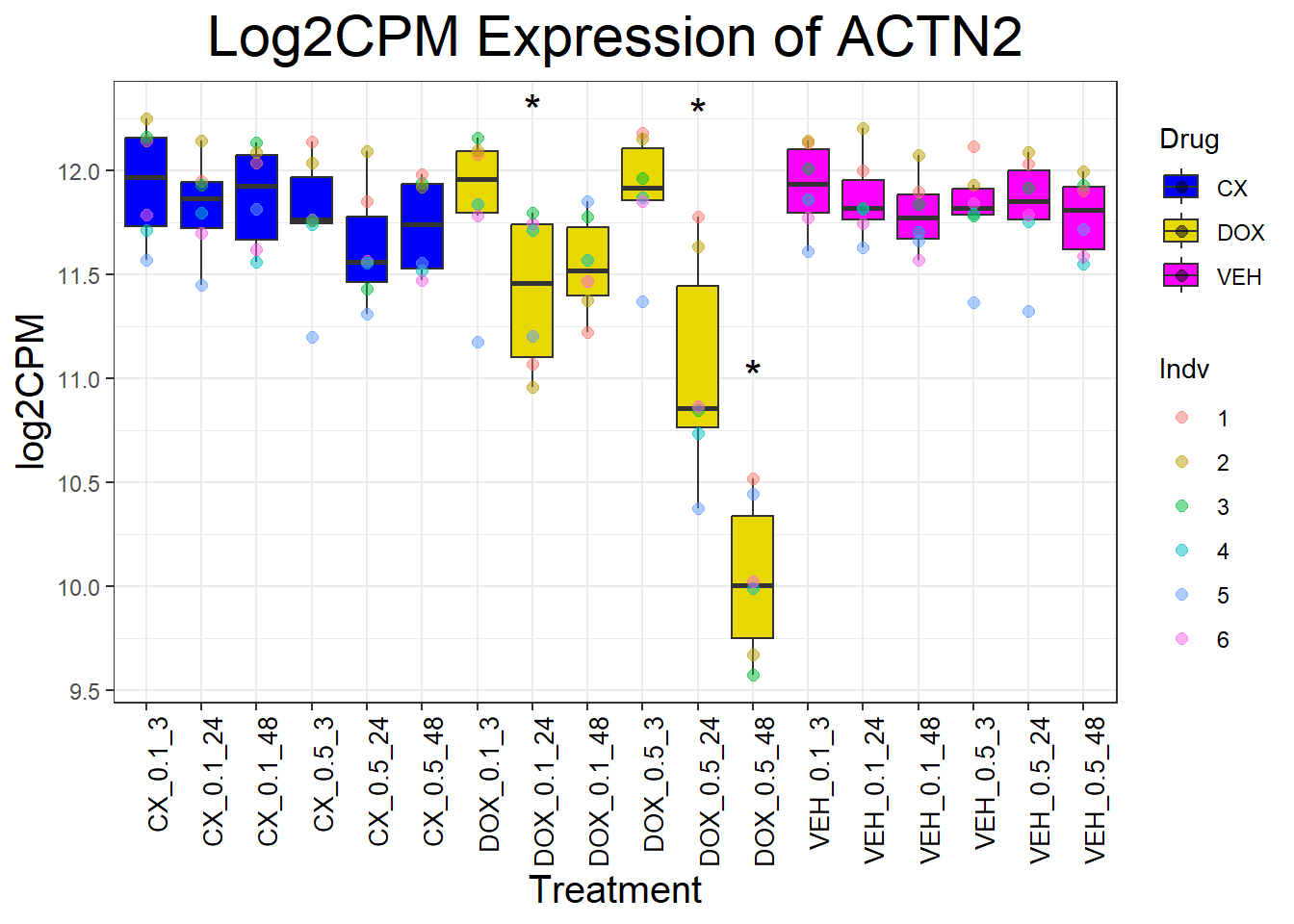
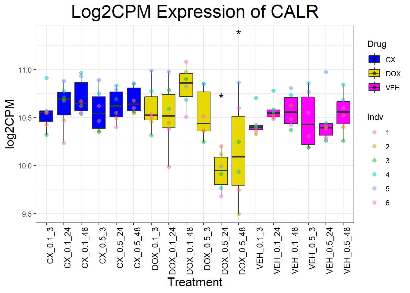
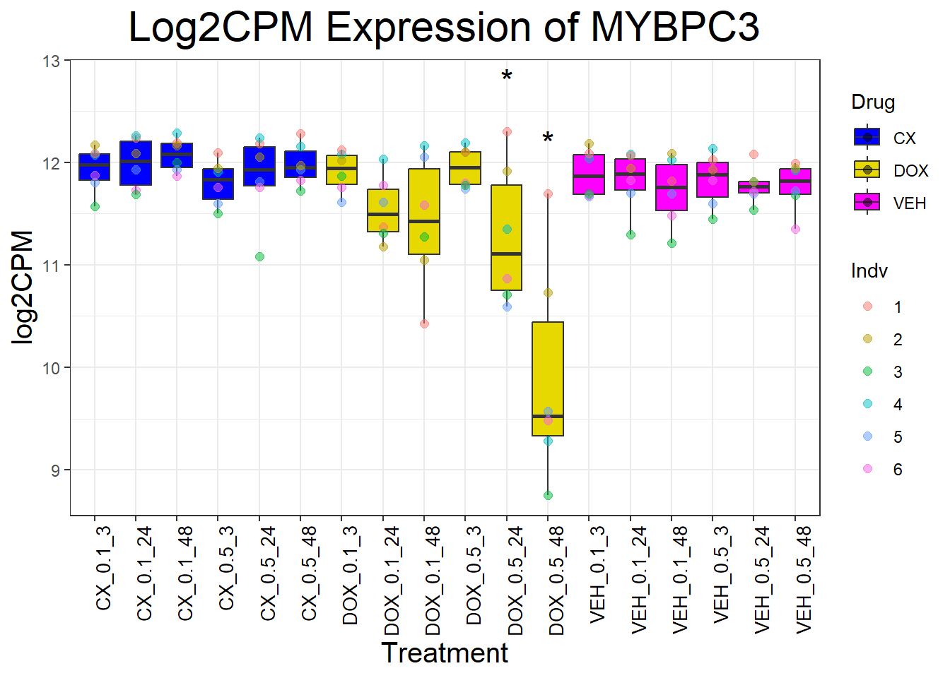
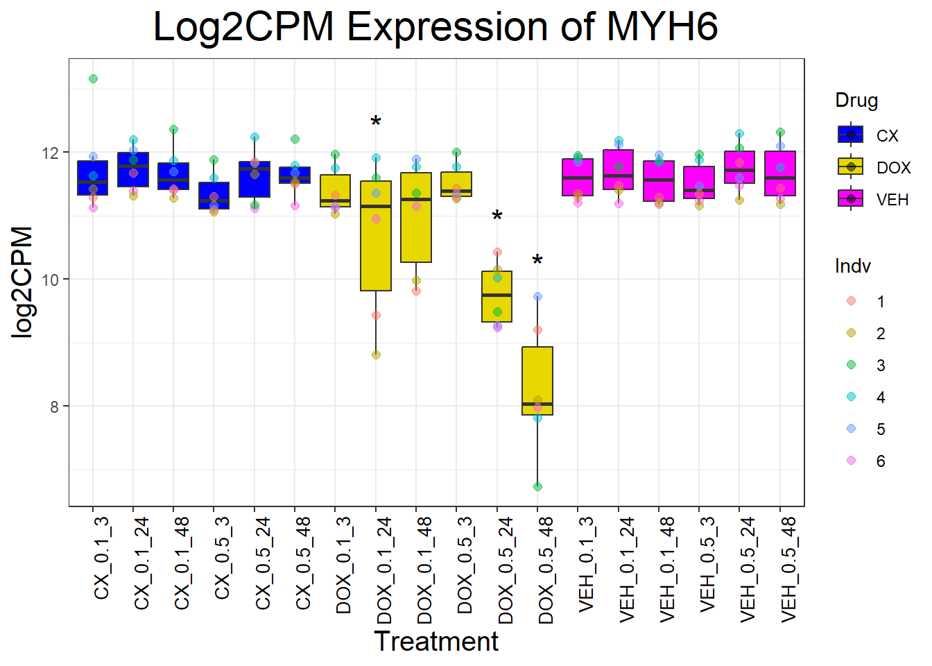
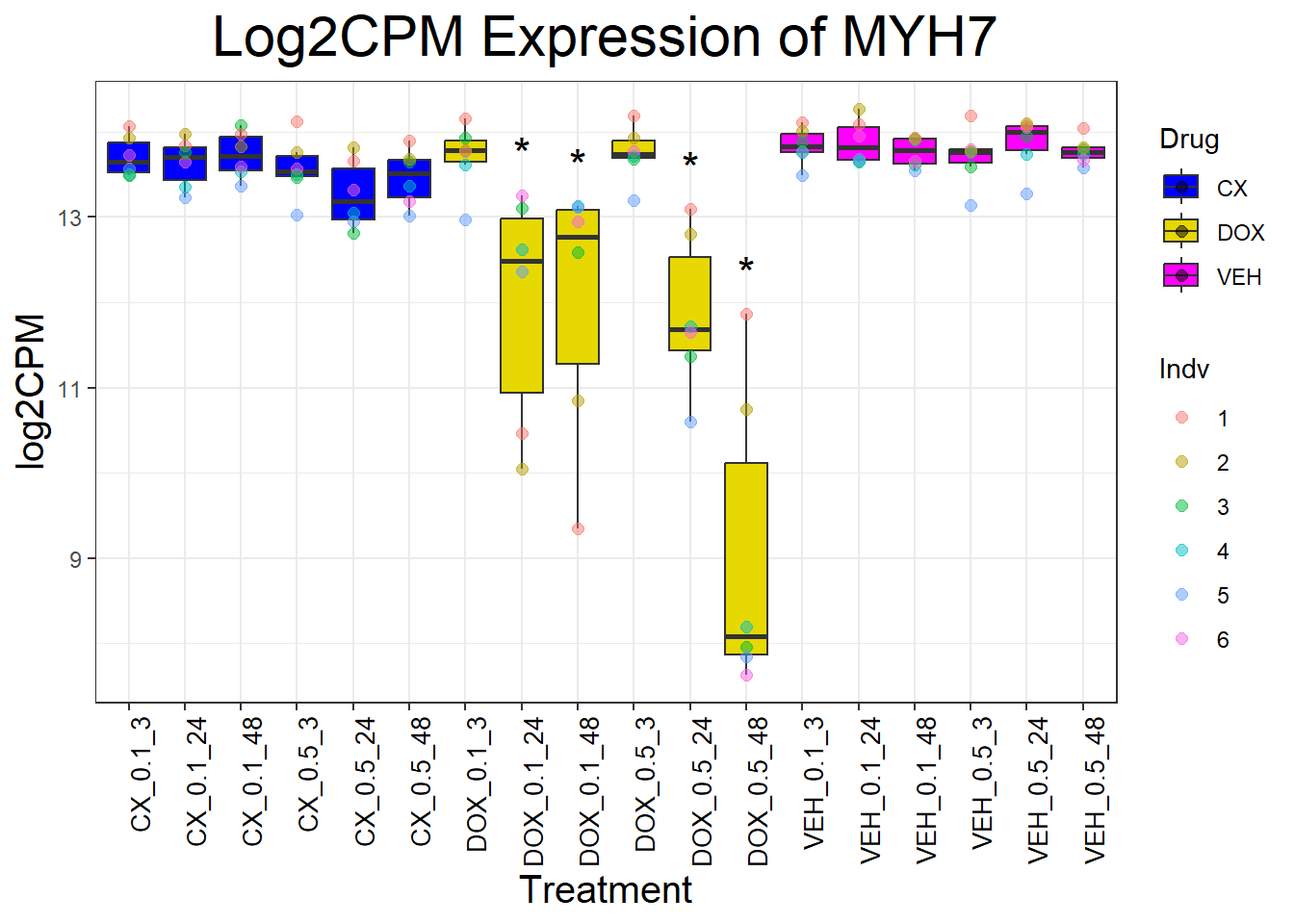
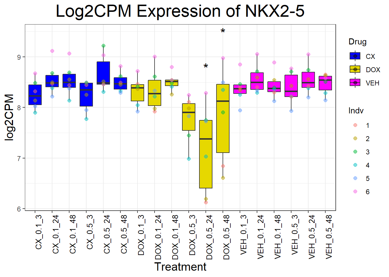
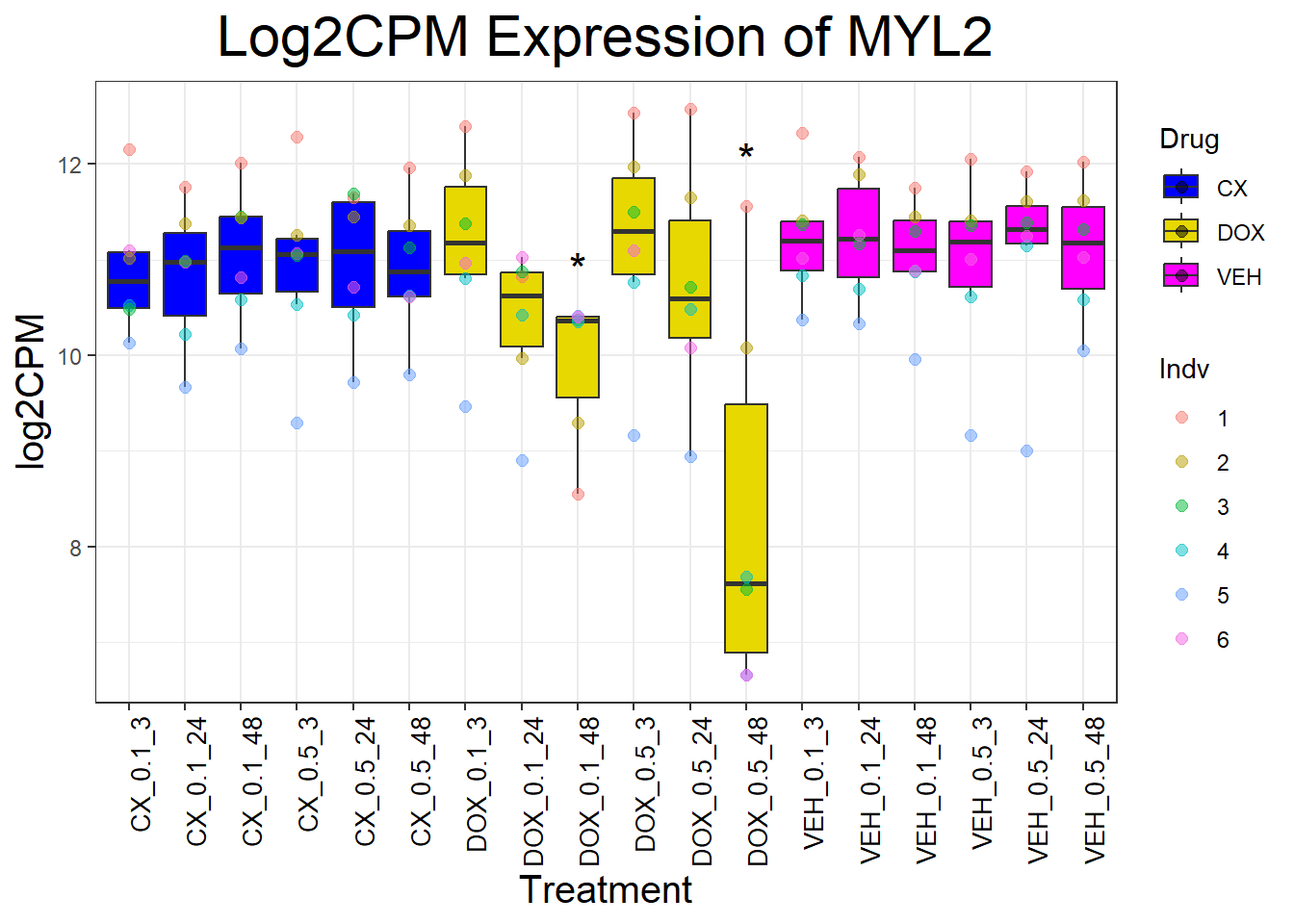
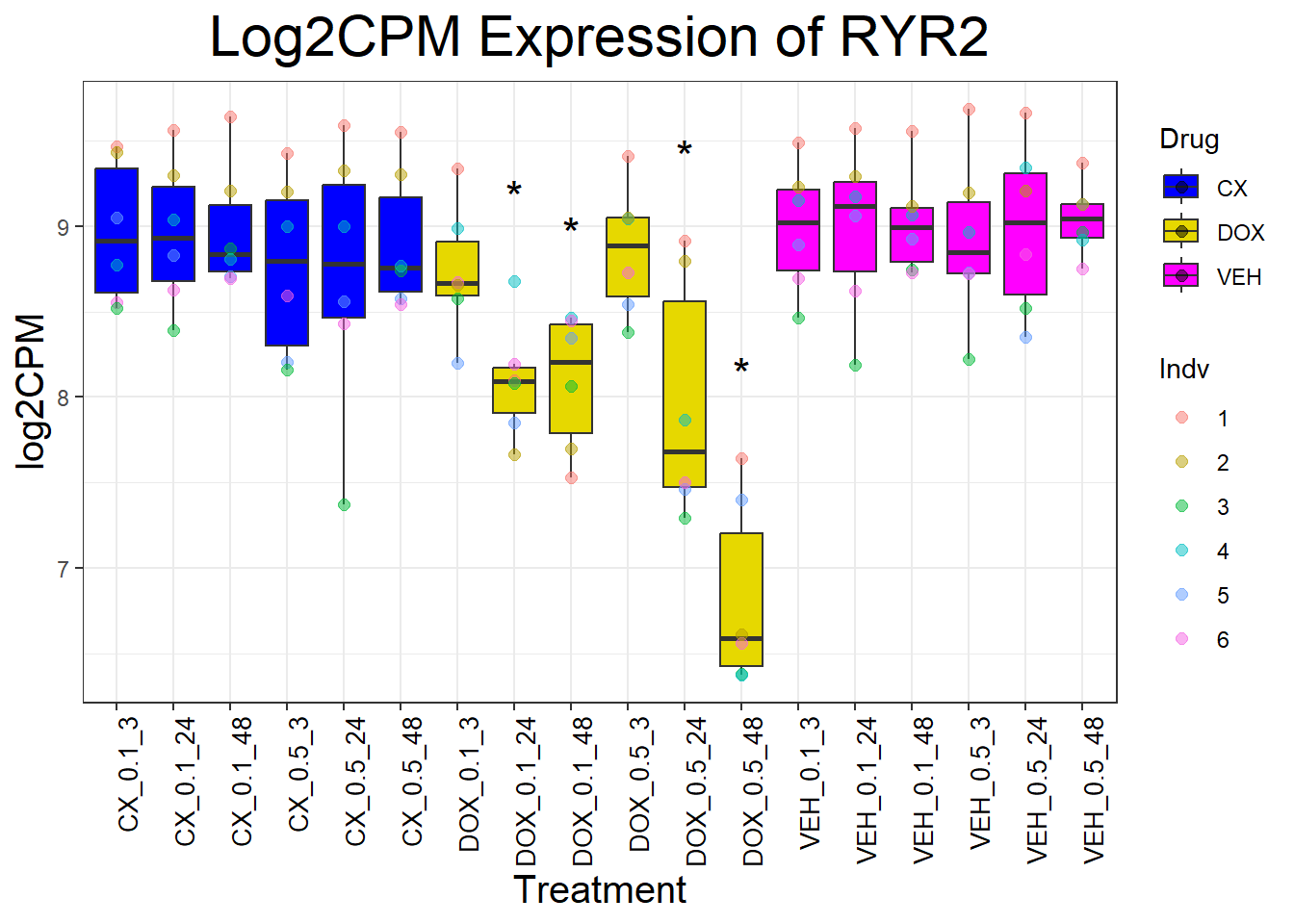
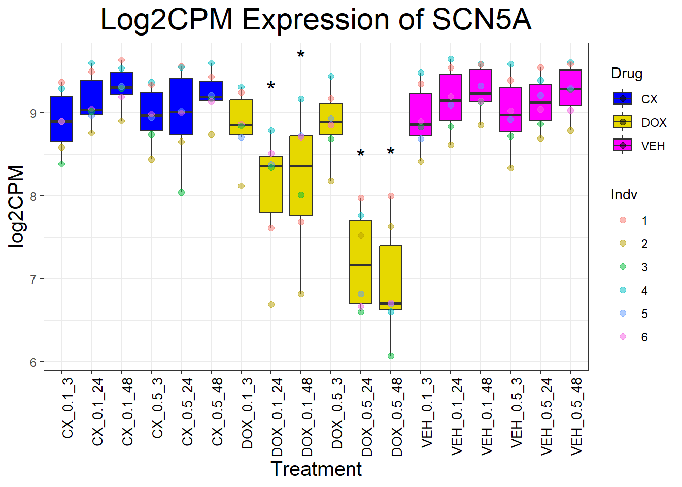
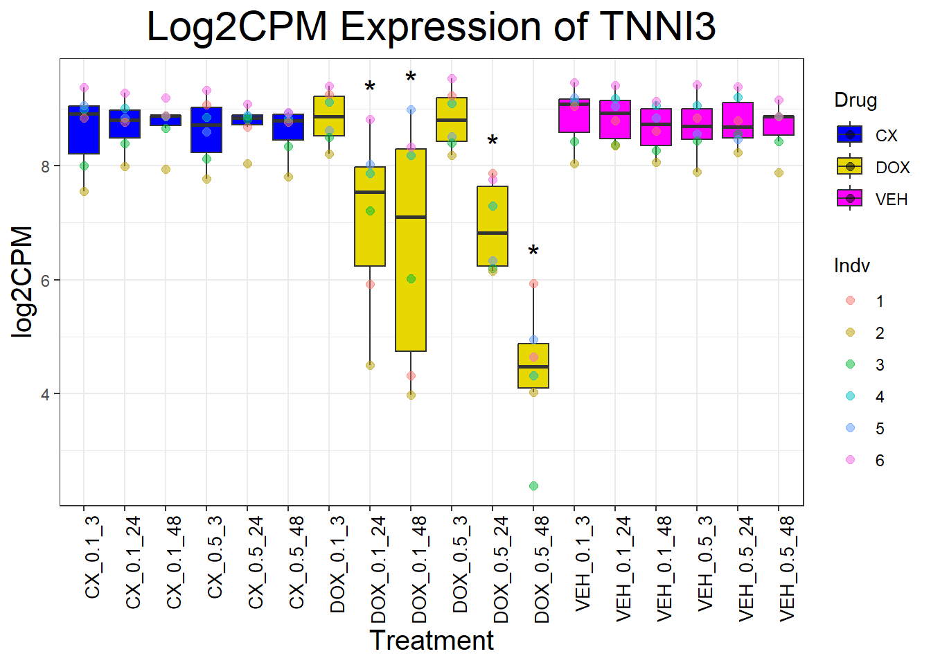
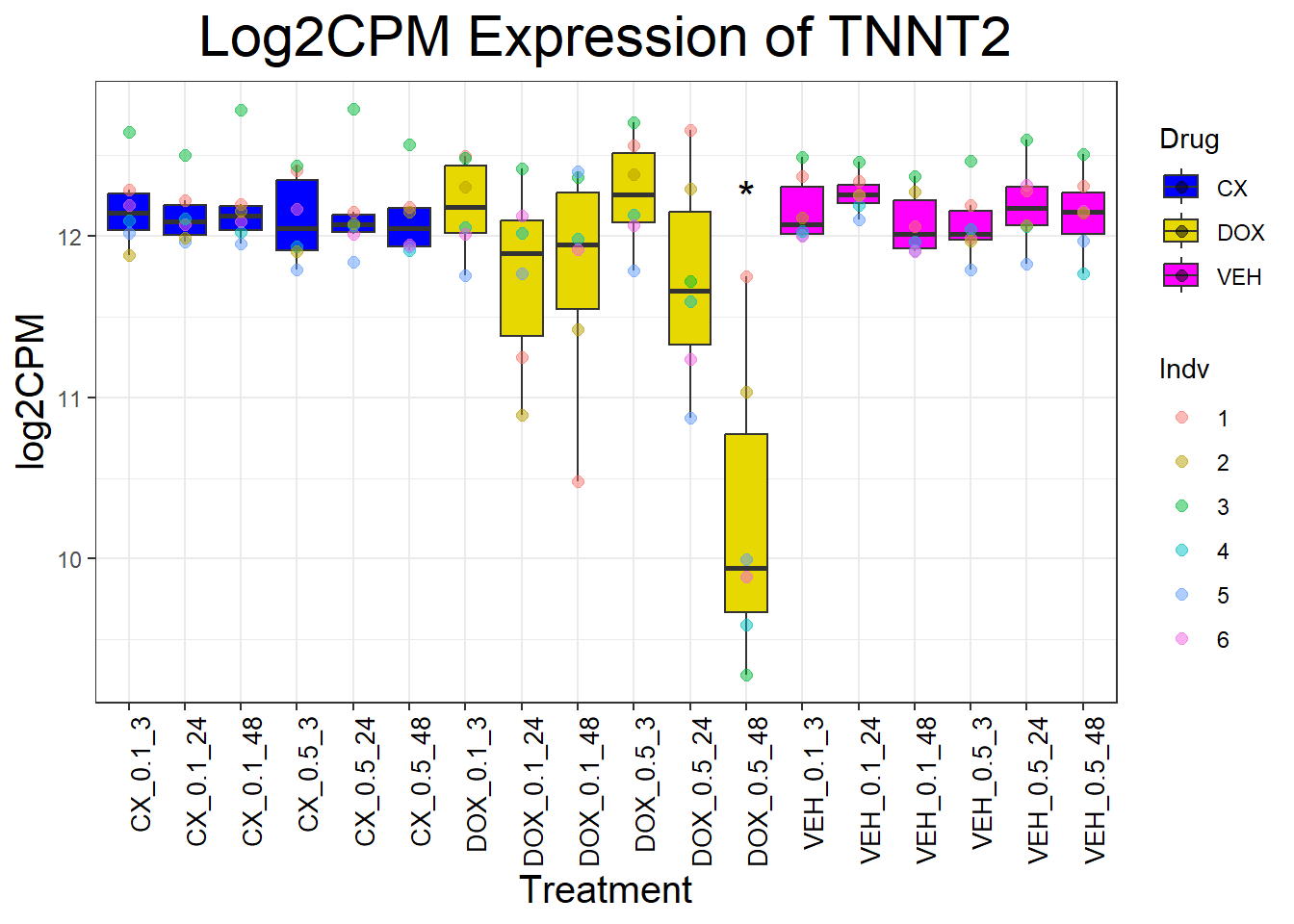
This analysis generates boxplots for cardiac genes and TOP2 genes across different treatments and timepoints.
📌 Load Required Libraries
library(ggplot2)
library(dplyr)
Warning: package 'dplyr' was built under R version 4.3.2library(tidyr)Warning: package 'tidyr' was built under R version 4.3.3library(org.Hs.eg.db)Warning: package 'AnnotationDbi' was built under R version 4.3.2Warning: package 'BiocGenerics' was built under R version 4.3.1Warning: package 'Biobase' was built under R version 4.3.1Warning: package 'IRanges' was built under R version 4.3.1Warning: package 'S4Vectors' was built under R version 4.3.2library(clusterProfiler)Warning: package 'clusterProfiler' was built under R version 4.3.3📌 Read Log2CPM Data
# Load feature count matrix
boxplot1 <- read.csv("data/Feature_count_Matrix_Log2CPM_filtered.csv") %>% as.data.frame()

# Ensure column names are cleaned
colnames(boxplot1) <- trimws(gsub("^X", "", colnames(boxplot1)))
📌 Define Genes of Interest
# Define the genes of interest
top2_genes <- c("TOP2A", "TOP2B")
cardiac_genes <- c("ACTN2", "CALR", "MYBPC3", "MYH6", "MYH7", "NKX2-5","MYL2", "RYR2", "SCN5A", "TNNI3", "TNNT2", "TTN")
dna_damage_genes <- c("TP53") # Using correct gene symbol TP53
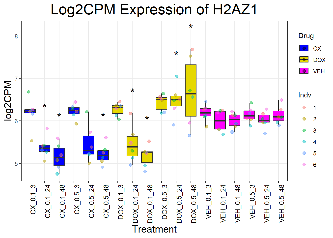
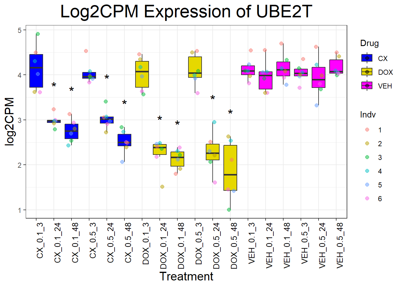
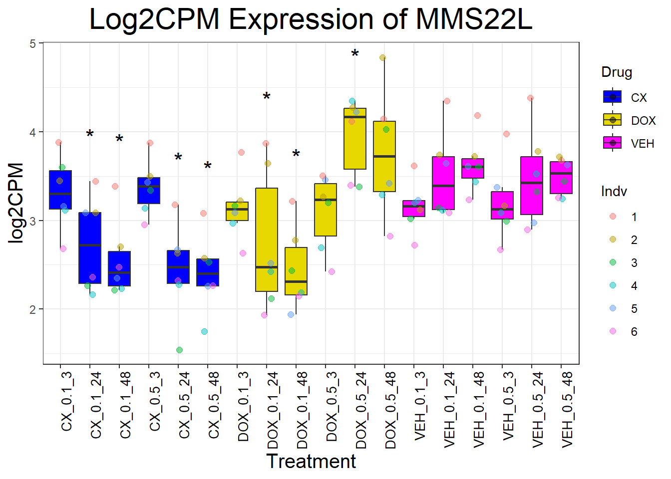
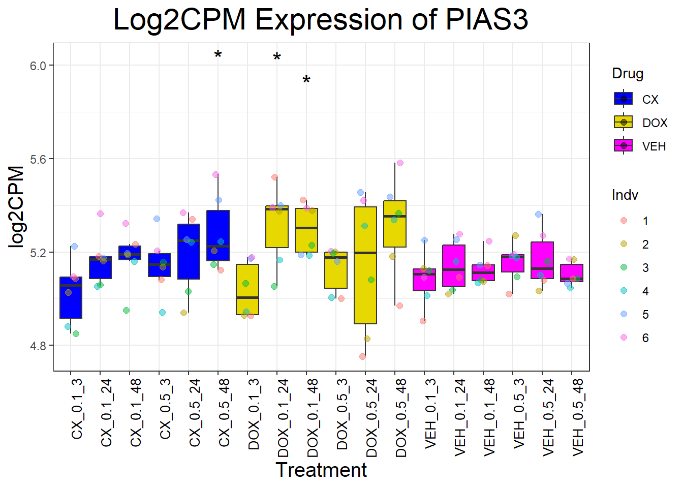
dna_repair_genes <- c("H2AZ1", "UBE2T", "MMS22L","PIAS3")
p53_target_genes <- c("IER5", "HHAT", "EPS8L2")📌 Read and Process DEGs Data
# Load Toptables
deg_files <- list.files("data/DEGs", pattern = "Toptable_.*\\.csv", full.names = TRUE)
deg_list <- lapply(deg_files, read.csv)
names(deg_list) <- gsub("data/DEGs/Toptable_|\\.csv", "", deg_files)

# Function to check significance based on **Entrez_ID in the correct sample**
is_significant <- function(gene, drug, conc, timepoint) {
  condition <- paste(drug, conc, timepoint, sep = "_")
  if (!condition %in% names(deg_list)) return(FALSE)

  toptable <- deg_list[[condition]]
  gene_entrez <- boxplot1$ENTREZID[boxplot1$SYMBOL == gene]

  if (length(gene_entrez) == 0) return(FALSE)

  return(any(gene_entrez %in% toptable$Entrez_ID[toptable$adj.P.Val < 0.05]))
}
📌 Process Data for Plotting
process_gene_data <- function(gene) {
  # Filter log2CPM data for the gene
  gene_data <- boxplot1 %>% filter(SYMBOL == gene)

  # Reshape data
  long_data <- gene_data %>%
    pivot_longer(cols = -c(ENTREZID, SYMBOL, GENENAME), names_to = "Sample", values_to = "log2CPM") %>%
    mutate(
      Indv = case_when(
        grepl("75.1", Sample) ~ "1",
        grepl("78.1", Sample) ~ "2",
        grepl("87.1", Sample) ~ "3",
        grepl("17.3", Sample) ~ "4",
        grepl("84.1", Sample) ~ "5",
        grepl("90.1", Sample) ~ "6",
        TRUE ~ NA_character_
      ),
      Drug = case_when(
        grepl("CX.5461", Sample) ~ "CX",
        grepl("DOX", Sample) ~ "DOX",
        grepl("VEH", Sample) ~ "VEH",
        TRUE ~ NA_character_
      ),
      Conc. = case_when(
        grepl("_0.1_", Sample) ~ "0.1",
        grepl("_0.5_", Sample) ~ "0.5",
        TRUE ~ NA_character_
      ),
      Timepoint = case_when(
        grepl("_3$", Sample) ~ "3",
        grepl("_24$", Sample) ~ "24",
        grepl("_48$", Sample) ~ "48",
        TRUE ~ NA_character_
      ),
      Condition = paste(Drug, Conc., Timepoint, sep = "_")
    )

  # **Ensure Condition is Ordered Correctly**
  long_data$Condition <- factor(
    long_data$Condition,
    levels = c(
      "CX_0.1_3", "CX_0.1_24", "CX_0.1_48", "CX_0.5_3", "CX_0.5_24", "CX_0.5_48",
      "DOX_0.1_3", "DOX_0.1_24", "DOX_0.1_48", "DOX_0.5_3", "DOX_0.5_24", "DOX_0.5_48",
      "VEH_0.1_3", "VEH_0.1_24", "VEH_0.1_48", "VEH_0.5_3", "VEH_0.5_24", "VEH_0.5_48"
    )
  )

  # Identify significant conditions **per Drug, Conc, and Timepoint**
  significance_labels <- long_data %>%
    distinct(Drug, Conc., Timepoint, Condition) %>%
    rowwise() %>%
    mutate(
      max_log2CPM = max(long_data$log2CPM[long_data$Condition == Condition], na.rm = TRUE),
      Significance = ifelse(is_significant(gene, Drug, Conc., Timepoint), "*", "")
    ) %>%
    filter(Significance != "") %>% ungroup()

  list(long_data = long_data, significance_labels = significance_labels)
}
📌Generate Boxplots for Cardiac Genes
for (gene in cardiac_genes) {
  data_info <- process_gene_data(gene)
  p <- ggplot(data_info$long_data, aes(x = Condition, y = log2CPM, fill = Drug)) +
    geom_boxplot(outlier.shape = NA) +
    scale_fill_manual(values = c("CX" = "#0000FF", "DOX" = "#e6d800", "VEH" = "#FF00FF")) +
    geom_point(aes(color = Indv), size = 2, alpha = 0.5, position = position_jitter(width = -1, height = 0)) +
    geom_text(data = data_info$significance_labels, aes(x = Condition, y = max_log2CPM + 0.5, label = Significance),
              inherit.aes = FALSE, size = 6, color = "black") +
    ggtitle(paste("Log2CPM Expression of", gene)) +
    labs(x = "Treatment", y = "log2CPM") +
    theme_bw() +
    theme(plot.title = element_text(size = rel(2), hjust = 0.5),
          axis.title = element_text(size = 15, color = "black"),
          axis.text.x = element_text(size = 10, color = "black", angle = 90, hjust = 1))

  print(p)
}

| Version | Author | Date |
|---|---|---|
| c8ef284 | sayanpaul01 | 2025-04-06 |
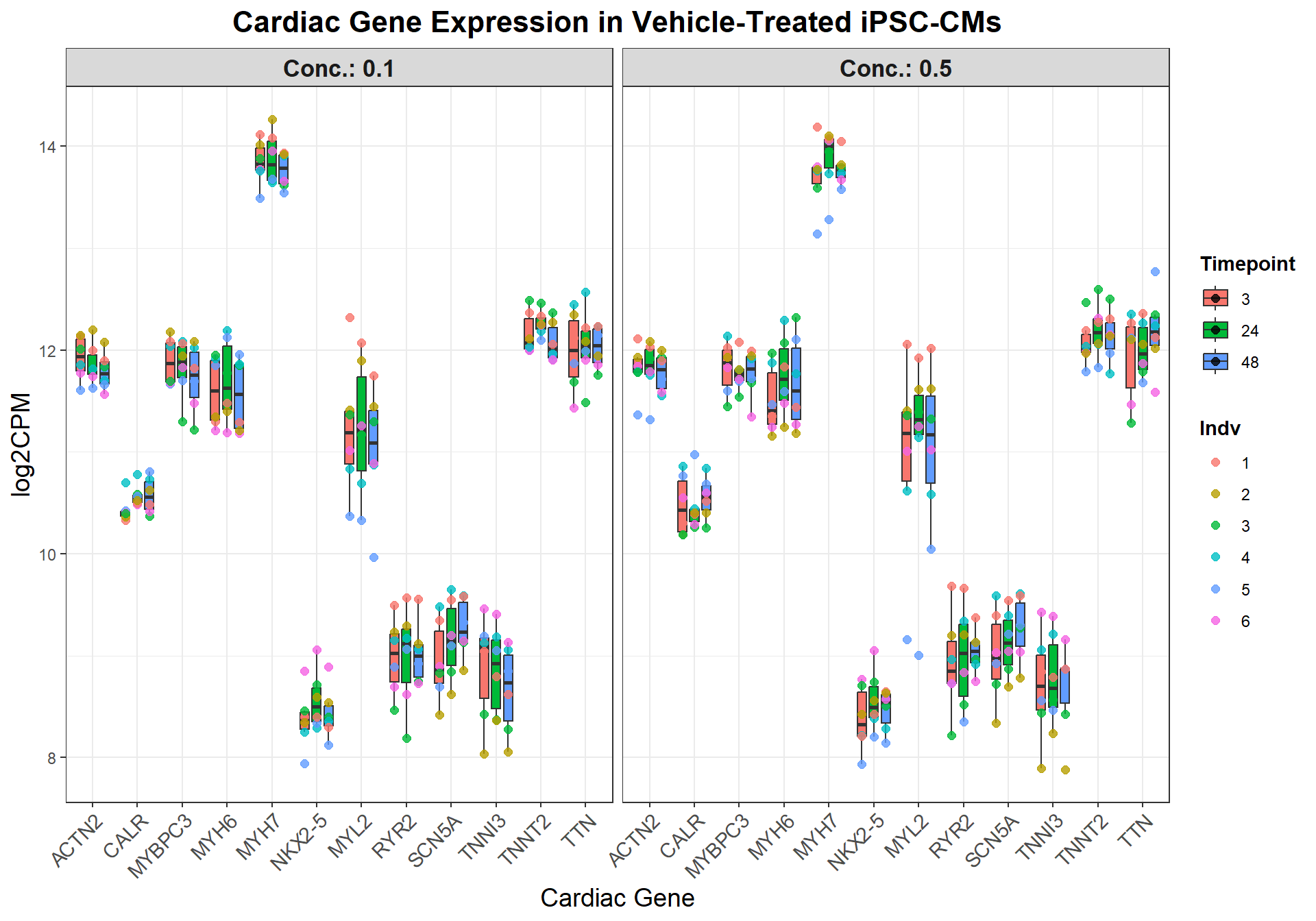
📌Generate Boxplots for Veh_Cardiac Genes
# 📌 Prepare data
cardiac_data <- boxplot1 %>%
  filter(SYMBOL %in% cardiac_genes) %>%
  pivot_longer(cols = -c(ENTREZID, SYMBOL, GENENAME), names_to = "Sample", values_to = "log2CPM") %>%
  mutate(
    Indv = case_when(
      grepl("75.1", Sample) ~ "1",
      grepl("78.1", Sample) ~ "2",
      grepl("87.1", Sample) ~ "3",
      grepl("17.3", Sample) ~ "4",
      grepl("84.1", Sample) ~ "5",
      grepl("90.1", Sample) ~ "6",
      TRUE ~ NA_character_
    ),
    Drug = case_when(
      grepl("CX.5461", Sample) ~ "CX",
      grepl("DOX", Sample) ~ "DOX",
      grepl("VEH", Sample) ~ "VEH",
      TRUE ~ NA_character_
    ),
    Conc. = case_when(
      grepl("_0.1_", Sample) ~ "0.1",
      grepl("_0.5_", Sample) ~ "0.5",
      TRUE ~ NA_character_
    ),
    Timepoint = case_when(
      grepl("_3$", Sample) ~ "3",
      grepl("_24$", Sample) ~ "24",
      grepl("_48$", Sample) ~ "48",
      TRUE ~ NA_character_
    )
  ) %>%
  filter(Drug == "VEH")

# 📌 Set factors
cardiac_data$SYMBOL <- factor(cardiac_data$SYMBOL, levels = cardiac_genes)
cardiac_data$Timepoint <- factor(cardiac_data$Timepoint, levels = c("3", "24", "48"))
cardiac_data$Conc. <- factor(cardiac_data$Conc., levels = c("0.1", "0.5"))

# Add a new combined X-axis label: Gene + Timepoint
cardiac_data <- cardiac_data %>%
  mutate(Gene_Time = interaction(SYMBOL, Timepoint, sep = "_"),
         SYMBOL = factor(SYMBOL, levels = cardiac_genes),
         Timepoint = factor(Timepoint, levels = c("3", "24", "48")),
         Conc. = factor(Conc., levels = c("0.1", "0.5")))

# Plot using Gene-Time combination for clean x-axis dodge
ggplot(cardiac_data, aes(x = SYMBOL, y = log2CPM, fill = Timepoint)) +
  geom_boxplot(
    aes(group = interaction(SYMBOL, Timepoint)),
    position = position_dodge(width = 0.8),
    outlier.shape = NA,
    width = 0.6
  ) +
  geom_point(
    aes(color = Indv, group = interaction(SYMBOL, Timepoint)),
    position = position_dodge(width = 0.8),
    size = 2,
    alpha = 0.8
  ) +
  facet_grid(. ~ Conc., labeller = label_both) +
  labs(
    title = "Cardiac Gene Expression in Vehicle-Treated iPSC-CMs",
    x = "Cardiac Gene",
    y = "log2CPM"
  ) +
  theme_bw() +
  theme(
    plot.title = element_text(size = 16, face = "bold", hjust = 0.5),
    axis.text.x = element_text(angle = 45, hjust = 1, size = 11),
    axis.title = element_text(size = 14),
    strip.text = element_text(size = 13, face = "bold"),
    legend.title = element_text(face = "bold"),
    legend.position = "right"
  )
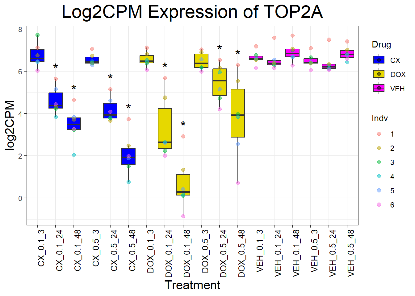
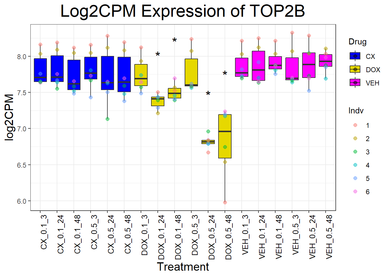
📌Generate Boxplots for TOP2 Genes
for (gene in top2_genes) {
  data_info <- process_gene_data(gene)
  p <- ggplot(data_info$long_data, aes(x = Condition, y = log2CPM, fill = Drug)) +
    geom_boxplot(outlier.shape = NA) +
    scale_fill_manual(values = c("CX" = "#0000FF", "DOX" = "#e6d800", "VEH" = "#FF00FF")) +
    geom_point(aes(color = Indv), size = 2, alpha = 0.5, position = position_jitter(width = -1, height = 0)) +
    geom_text(data = data_info$significance_labels, aes(x = Condition, y = max_log2CPM + 0.5, label = Significance),
              inherit.aes = FALSE, size = 6, color = "black") +
    ggtitle(paste("Log2CPM Expression of", gene)) +
    labs(x = "Treatment", y = "log2CPM") +
    theme_bw() +
    theme(plot.title = element_text(size = rel(2), hjust = 0.5),
          axis.title = element_text(size = 15, color = "black"),
          axis.text.x = element_text(size = 10, color = "black", angle = 90, hjust = 1))

  print(p)
}
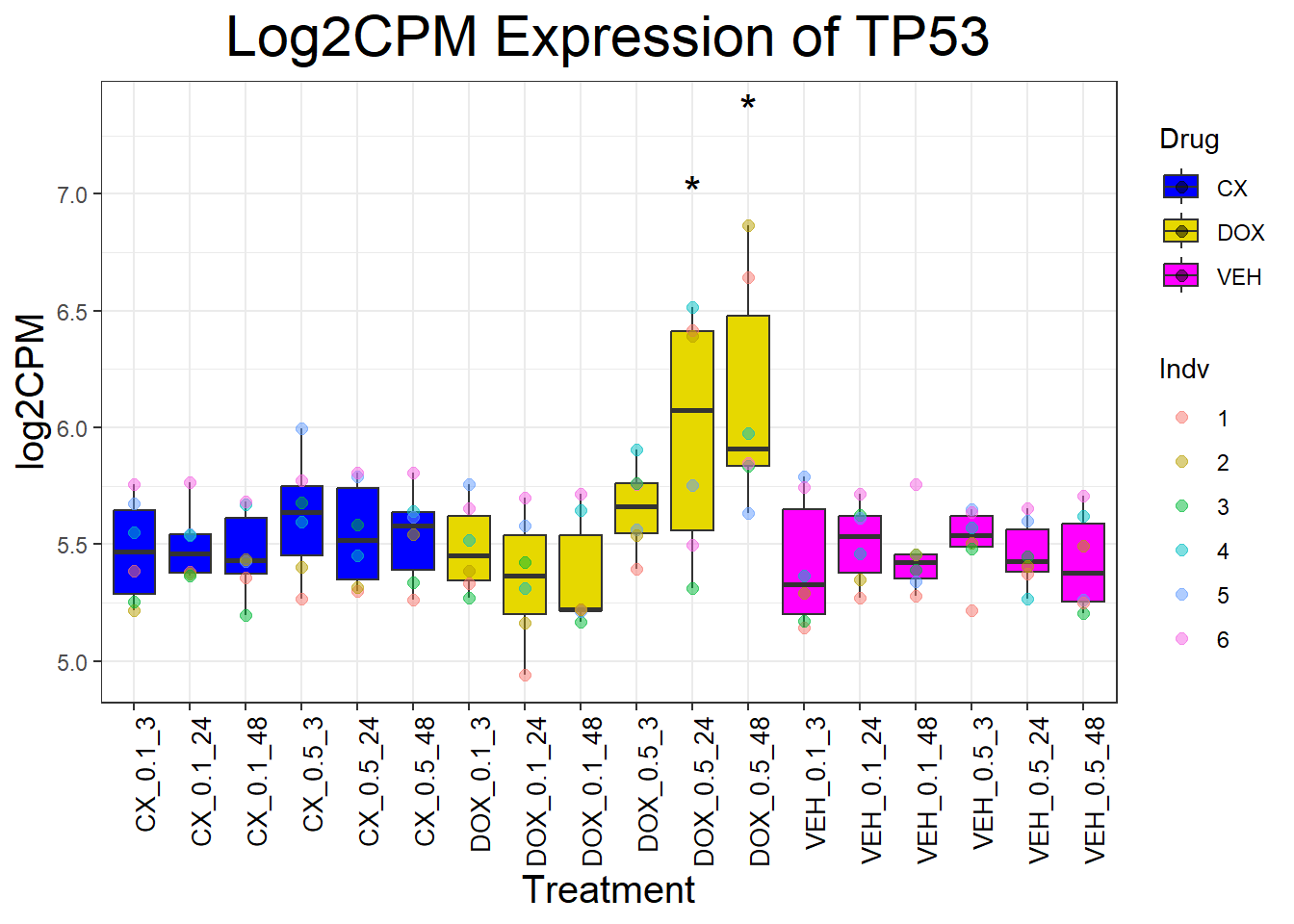
📌 Generate Boxplots for TP53 Genes
for (gene in dna_damage_genes) {
  data_info <- process_gene_data(gene)
  p <- ggplot(data_info$long_data, aes(x = Condition, y = log2CPM, fill = Drug)) +
    geom_boxplot(outlier.shape = NA) +
    scale_fill_manual(values = c("CX" = "#0000FF", "DOX" = "#e6d800", "VEH" = "#FF00FF")) +
    geom_point(aes(color = Indv), size = 2, alpha = 0.5, position = position_jitter(width = -1, height = 0)) +
    geom_text(data = data_info$significance_labels, aes(x = Condition, y = max_log2CPM + 0.5, label = Significance),
              inherit.aes = FALSE, size = 6, color = "black") +
    ggtitle(paste("Log2CPM Expression of", gene)) +
    labs(x = "Treatment", y = "log2CPM") +
    theme_bw() +
    theme(plot.title = element_text(size = rel(2), hjust = 0.5),
          axis.title = element_text(size = 15, color = "black"),
          axis.text.x = element_text(size = 10, color = "black", angle = 90, hjust = 1))

  print(p)
}
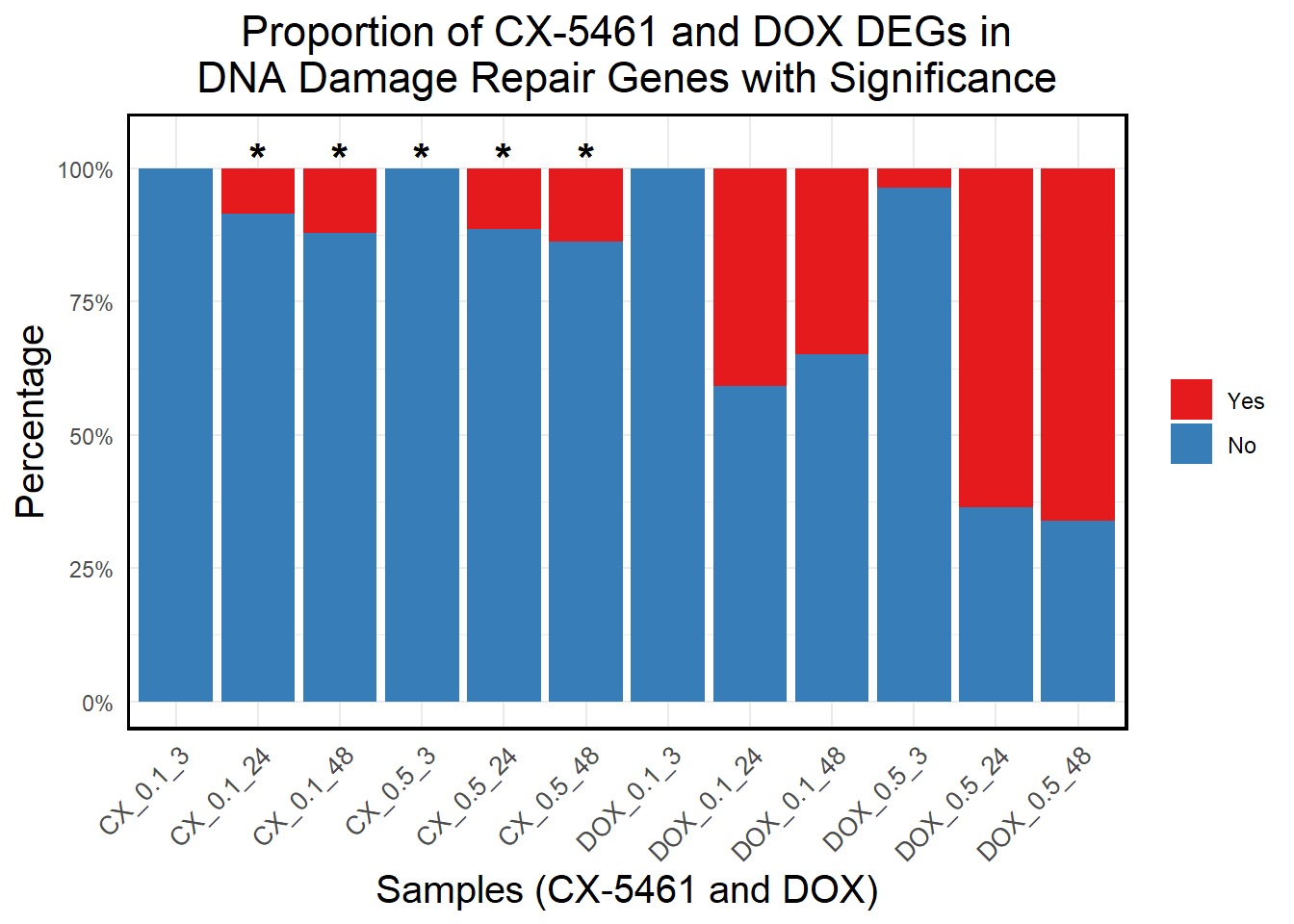
##📌 DNA Damage Repair Genes Proportion
📌 Read and Process DEG Data
# Load DEGs Data
CX_0.1_3 <- read.csv("data/DEGs/Toptable_CX_0.1_3.csv")
CX_0.1_24 <- read.csv("data/DEGs/Toptable_CX_0.1_24.csv")
CX_0.1_48 <- read.csv("data/DEGs/Toptable_CX_0.1_48.csv")
CX_0.5_3 <- read.csv("data/DEGs/Toptable_CX_0.5_3.csv")
CX_0.5_24 <- read.csv("data/DEGs/Toptable_CX_0.5_24.csv")
CX_0.5_48 <- read.csv("data/DEGs/Toptable_CX_0.5_48.csv")

DOX_0.1_3 <- read.csv("data/DEGs/Toptable_DOX_0.1_3.csv")
DOX_0.1_24 <- read.csv("data/DEGs/Toptable_DOX_0.1_24.csv")
DOX_0.1_48 <- read.csv("data/DEGs/Toptable_DOX_0.1_48.csv")
DOX_0.5_3 <- read.csv("data/DEGs/Toptable_DOX_0.5_3.csv")
DOX_0.5_24 <- read.csv("data/DEGs/Toptable_DOX_0.5_24.csv")
DOX_0.5_48 <- read.csv("data/DEGs/Toptable_DOX_0.5_48.csv")

# Extract Significant DEGs
DEGs <- list(
  "CX_0.1_3" = CX_0.1_3$Entrez_ID[CX_0.1_3$adj.P.Val < 0.05],
  "CX_0.1_24" = CX_0.1_24$Entrez_ID[CX_0.1_24$adj.P.Val < 0.05],
  "CX_0.1_48" = CX_0.1_48$Entrez_ID[CX_0.1_48$adj.P.Val < 0.05],
  "CX_0.5_3" = CX_0.5_3$Entrez_ID[CX_0.5_3$adj.P.Val < 0.05],
  "CX_0.5_24" = CX_0.5_24$Entrez_ID[CX_0.5_24$adj.P.Val < 0.05],
  "CX_0.5_48" = CX_0.5_48$Entrez_ID[CX_0.5_48$adj.P.Val < 0.05],
  "DOX_0.1_3" = DOX_0.1_3$Entrez_ID[DOX_0.1_3$adj.P.Val < 0.05],
  "DOX_0.1_24" = DOX_0.1_24$Entrez_ID[DOX_0.1_24$adj.P.Val < 0.05],
  "DOX_0.1_48" = DOX_0.1_48$Entrez_ID[DOX_0.1_48$adj.P.Val < 0.05],
  "DOX_0.5_3" = DOX_0.5_3$Entrez_ID[DOX_0.5_3$adj.P.Val < 0.05],
  "DOX_0.5_24" = DOX_0.5_24$Entrez_ID[DOX_0.5_24$adj.P.Val < 0.05],
  "DOX_0.5_48" = DOX_0.5_48$Entrez_ID[DOX_0.5_48$adj.P.Val < 0.05]
)

# Extract Significant DEGs
DEG1 <- CX_0.1_3$Entrez_ID[CX_0.1_3$adj.P.Val < 0.05]
DEG2 <- CX_0.1_24$Entrez_ID[CX_0.1_24$adj.P.Val < 0.05]
DEG3 <- CX_0.1_48$Entrez_ID[CX_0.1_48$adj.P.Val < 0.05]
DEG4 <- CX_0.5_3$Entrez_ID[CX_0.5_3$adj.P.Val < 0.05]
DEG5 <- CX_0.5_24$Entrez_ID[CX_0.5_24$adj.P.Val < 0.05]
DEG6 <- CX_0.5_48$Entrez_ID[CX_0.5_48$adj.P.Val < 0.05]

DEG7 <- DOX_0.1_3$Entrez_ID[DOX_0.1_3$adj.P.Val < 0.05]
DEG8 <- DOX_0.1_24$Entrez_ID[DOX_0.1_24$adj.P.Val < 0.05]
DEG9 <- DOX_0.1_48$Entrez_ID[DOX_0.1_48$adj.P.Val < 0.05]
DEG10 <- DOX_0.5_3$Entrez_ID[DOX_0.5_3$adj.P.Val < 0.05]
DEG11 <- DOX_0.5_24$Entrez_ID[DOX_0.5_24$adj.P.Val < 0.05]
DEG12 <- DOX_0.5_48$Entrez_ID[DOX_0.5_48$adj.P.Val < 0.05]
📌 DNA Damage Repair Proportion with Chi-Square Test
# Read DNA Damage Genes List
DNA_damage <- read.csv("data/DNA_Damage.csv", stringsAsFactors = FALSE)

# Convert gene symbols to Entrez IDs
DNA_damage <- DNA_damage %>%
  mutate(Entrez_ID = mapIds(org.Hs.eg.db,
                            keys = Symbol,
                            column = "ENTREZID",
                            keytype = "SYMBOL",
                            multiVals = "first"))

# Extract DNA damage gene Entrez IDs
DNA_damage_genes <- na.omit(DNA_damage$Entrez_ID)
total_DNA_damage_genes <- length(DNA_damage_genes)  # Total number of DNA damage genes

# Define CX-5461 DEG lists
CX_DEGs <- list(
  "CX_0.1_3" = DEG1, "CX_0.1_24" = DEG2, "CX_0.1_48" = DEG3,
  "CX_0.5_3" = DEG4, "CX_0.5_24" = DEG5, "CX_0.5_48" = DEG6
)

# Define DOX DEG lists
DOX_DEGs <- list(
  "DOX_0.1_3" = DEG7, "DOX_0.1_24" = DEG8, "DOX_0.1_48" = DEG9,
  "DOX_0.5_3" = DEG10, "DOX_0.5_24" = DEG11, "DOX_0.5_48" = DEG12
)

# Function to calculate the presence of DNA damage genes in DEGs
calculate_proportion <- function(deg_list, drug_name) {
  data.frame(
    Sample = names(deg_list),
    Drug = drug_name,
    DNA_Damage_DEGs = sapply(deg_list, function(ids) sum(ids %in% DNA_damage_genes)),  # DEGs present in DNA damage set
    Non_DNA_Damage_DEGs = sapply(deg_list, function(ids) total_DNA_damage_genes - sum(ids %in% DNA_damage_genes))  # Remaining DNA damage genes
  ) %>%
    mutate(
      Yes_Proportion = (DNA_Damage_DEGs / total_DNA_damage_genes) * 100,  # Percentage of DEGs in DNA damage genes
      No_Proportion = (Non_DNA_Damage_DEGs / total_DNA_damage_genes) * 100  # Remaining DNA damage genes as No
    )
}

# Calculate proportions for CX-5461 and DOX
CX_proportion <- calculate_proportion(CX_DEGs, "CX-5461")
DOX_proportion <- calculate_proportion(DOX_DEGs, "DOX")

# Combine data
proportion_data <- bind_rows(CX_proportion, DOX_proportion)

# Convert to long format for stacked bar plot
proportion_long <- proportion_data %>%
  select(Sample, Drug, Yes_Proportion, No_Proportion) %>%
  pivot_longer(cols = c(Yes_Proportion, No_Proportion), names_to = "Category", values_to = "Percentage") %>%
  mutate(Category = ifelse(Category == "Yes_Proportion", "Yes", "No"))

# **Ensure correct order of samples on X-axis**
sample_order <- c(
  "CX_0.1_3", "CX_0.1_24", "CX_0.1_48", "CX_0.5_3", "CX_0.5_24", "CX_0.5_48",
  "DOX_0.1_3", "DOX_0.1_24", "DOX_0.1_48", "DOX_0.5_3", "DOX_0.5_24", "DOX_0.5_48"
)
proportion_long$Sample <- factor(proportion_long$Sample, levels = sample_order, ordered = TRUE)

# **Fix: Ensure "Yes" is on top and "No" is at the bottom in stacked bars**
proportion_long$Category <- factor(proportion_long$Category, levels = c("Yes", "No"))  # Ensures "Yes" on top, "No" at bottom

# **Perform Chi-Square Test for CX vs DOX at each timepoint**
chi_square_results <- data.frame(Sample = character(), P_Value = numeric())

for (i in seq(1, 6)) {  # Pairwise comparison (CX vs DOX)
  cx_sample <- sample_order[i]
  dox_sample <- sample_order[i + 6]  # Matches CX_0.1_3 with DOX_0.1_3, etc.

  cx_data <- filter(proportion_data, Sample == cx_sample)
  dox_data <- filter(proportion_data, Sample == dox_sample)

  # Construct contingency table for Chi-Square test
  contingency_table <- matrix(
    c(cx_data$DNA_Damage_DEGs, cx_data$Non_DNA_Damage_DEGs,
      dox_data$DNA_Damage_DEGs, dox_data$Non_DNA_Damage_DEGs),
    nrow = 2, byrow = TRUE
  )

  # Run Chi-Square Test
  test_result <- chisq.test(contingency_table)
  p_value <- test_result$p.value

  # Store results
  chi_square_results <- rbind(chi_square_results, data.frame(Sample = cx_sample, P_Value = p_value))
}

# Add significance stars
chi_square_results$Significant <- ifelse(chi_square_results$P_Value < 0.05, "*", "")

# Merge Chi-Square results
proportion_long <- left_join(proportion_long, chi_square_results, by = "Sample")

# **Save output**
write.csv(proportion_long, "C:/Work/Postdoc_UTMB/CX-5461 Project/Transcriptome literatures/lit2/Proportion_Stacked_DNA_Damage_DEGs_with_ChiSquare.csv", row.names = FALSE)


# Define correct factor orders for samples
sample_order <- c(
  "CX_0.1_3", "CX_0.1_24", "CX_0.1_48", "CX_0.5_3", "CX_0.5_24", "CX_0.5_48",
  "DOX_0.1_3", "DOX_0.1_24", "DOX_0.1_48", "DOX_0.5_3", "DOX_0.5_24", "DOX_0.5_48"
)

# Reapply factor levels for correct order in both proportion_data and proportion_long
proportion_data$Sample <- factor(proportion_data$Sample, levels = sample_order, ordered = TRUE)
proportion_long$Sample <- factor(proportion_long$Sample, levels = sample_order, ordered = TRUE)

# **Fix: Ensure "Yes" is on top and "No" is at the bottom in stacked bars**
proportion_long$Category <- factor(proportion_long$Category, levels = c("Yes", "No"))
📌 DNA Damage Repair Proportion Plot
# **Generate Stacked Bar Plot with Correct X-Axis Order**
ggplot(proportion_long, aes(x = Sample, y = Percentage, fill = Category)) +
  geom_bar(stat = "identity", position = "stack") +  # Stacked bars
  geom_text(data = subset(proportion_long, Significant == "*"),
            aes(x = Sample, y = 102, label = "*"),  # Position stars slightly above 100%
            size = 6, color = "black", fontface = "bold") +
  scale_y_continuous(labels = scales::percent_format(scale = 1), limits = c(0, 105)) +  # Increase Y-axis slightly
  scale_fill_manual(values = c("Yes" = "#e41a1c", "No" = "#377eb8")) +  # Yes (Red), No (Blue)
  labs(
    title = "Proportion of CX-5461 and DOX DEGs in\nDNA Damage Repair Genes with Significance",
    x = "Samples (CX-5461 and DOX)",
    y = "Percentage",
    fill = "Category"
  ) +
  theme_minimal() +
  theme(
    plot.title = element_text(size = rel(1.5), hjust = 0.5),
    axis.title = element_text(size = 15, color = "black"),
    axis.text.x = element_text(size = 10, angle = 45, hjust = 1),
    legend.title = element_blank(),
    panel.border = element_rect(color = "black", fill = NA, linewidth = 1.2),
    strip.background = element_blank(),
    strip.text = element_text(size = 12, face = "bold")
  )
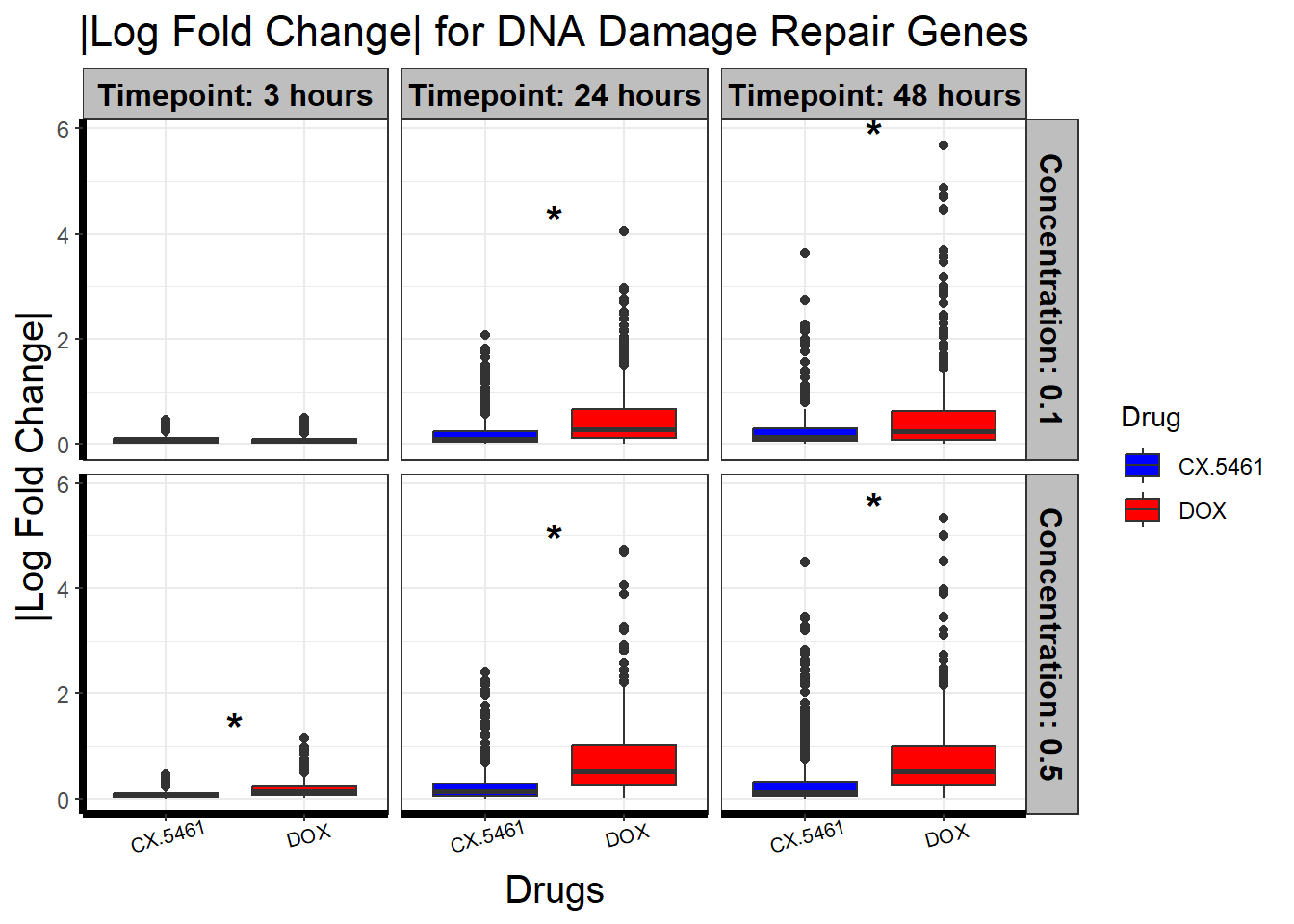
📌 DNA Damage Repair abs logFC distribution
# Load necessary libraries
library(dplyr)
library(ggplot2)
library(tidyr)
library(org.Hs.eg.db)
library(rstatix)
Warning: package 'rstatix' was built under R version 4.3.1# Read DNA Damage Response Gene List
DNA_damage <- read.csv("data/DNA_Damage.csv", stringsAsFactors = FALSE)
# Convert gene symbols to Entrez IDs
DNA_damage <- DNA_damage %>%
mutate(Entrez_ID = mapIds(org.Hs.eg.db,
keys = Symbol,
column = "ENTREZID",
keytype = "SYMBOL",
multiVals = "first"))
DNA_damage_genes <- na.omit(DNA_damage$Entrez_ID)
all_toptables <- bind_rows(
CX_0.1_3 %>% mutate(Drug = "CX.5461", Concentration = 0.1, Timepoint = "3"),
CX_0.1_24 %>% mutate(Drug = "CX.5461", Concentration = 0.1, Timepoint = "24"),
CX_0.1_48 %>% mutate(Drug = "CX.5461", Concentration = 0.1, Timepoint = "48"),
CX_0.5_3 %>% mutate(Drug = "CX.5461", Concentration = 0.5, Timepoint = "3"),
CX_0.5_24 %>% mutate(Drug = "CX.5461", Concentration = 0.5, Timepoint = "24"),
CX_0.5_48 %>% mutate(Drug = "CX.5461", Concentration = 0.5, Timepoint = "48"),
DOX_0.1_3 %>% mutate(Drug = "DOX", Concentration = 0.1, Timepoint = "3"),
DOX_0.1_24 %>% mutate(Drug = "DOX", Concentration = 0.1, Timepoint = "24"),
DOX_0.1_48 %>% mutate(Drug = "DOX", Concentration = 0.1, Timepoint = "48"),
DOX_0.5_3 %>% mutate(Drug = "DOX", Concentration = 0.5, Timepoint = "3"),
DOX_0.5_24 %>% mutate(Drug = "DOX", Concentration = 0.5, Timepoint = "24"),
DOX_0.5_48 %>% mutate(Drug = "DOX", Concentration = 0.5, Timepoint = "48")
)
filtered_toptables <- all_toptables %>%
filter(Entrez_ID %in% DNA_damage_genes) %>%
mutate(abs_logFC = abs(logFC))
filtered_toptables <- filtered_toptables %>%
mutate(
Drug = factor(Drug, levels = c("CX.5461", "DOX")), # CX first
Timepoint = factor(Timepoint, levels = c("3", "24", "48"),
labels = c("Timepoint: 3 hours", "Timepoint: 24 hours", "Timepoint: 48 hours")),
Concentration = factor(Concentration, levels = c(0.1, 0.5),
labels = c("Concentration: 0.1", "Concentration: 0.5"))
)
wilcox_results <- filtered_toptables %>%
group_by(Timepoint, Concentration) %>%
wilcox_test(abs_logFC ~ Drug) %>%
adjust_pvalue(method = "bonferroni") %>%
mutate(significance = ifelse(p < 0.05, "*", ""))
star_positions <- filtered_toptables %>%
group_by(Timepoint, Concentration, Drug) %>%
summarise(y_pos = max(abs_logFC, na.rm = TRUE) + 0.2, .groups = "drop") %>%
group_by(Timepoint, Concentration) %>%
summarise(y_pos = max(y_pos), .groups = "drop")
wilcox_results_plot <- wilcox_results %>%
left_join(star_positions, by = c("Timepoint", "Concentration")) %>%
mutate(x_position = 1.5) # Place stars in the middle between CX & DOX
ggplot(filtered_toptables, aes(x = Drug, y = abs_logFC, fill = Drug)) +
geom_boxplot() +
scale_fill_manual(values = c("CX.5461" = "blue", "DOX" = "red")) +
facet_grid(Concentration ~ Timepoint) +
geom_text(
data = wilcox_results_plot,
aes(x = x_position, y = y_pos, label = significance),
size = 6, fontface = "bold", color = "black", inherit.aes = FALSE
) +
theme_bw() +
xlab("Drugs") +
ylab("|Log Fold Change|") +
ggtitle("|Log Fold Change| for DNA Damage Repair Genes") +
theme(
plot.title = element_text(size = rel(1.5), hjust = 0.5),
axis.title = element_text(size = 15, color = "black"),
axis.line = element_line(linewidth = 1.5),
strip.background = element_rect(fill = "gray"),
strip.text = element_text(size = 12, color = "black", face = "bold"),
axis.text.x = element_text(size = 8, color = "black", angle = 15)
)
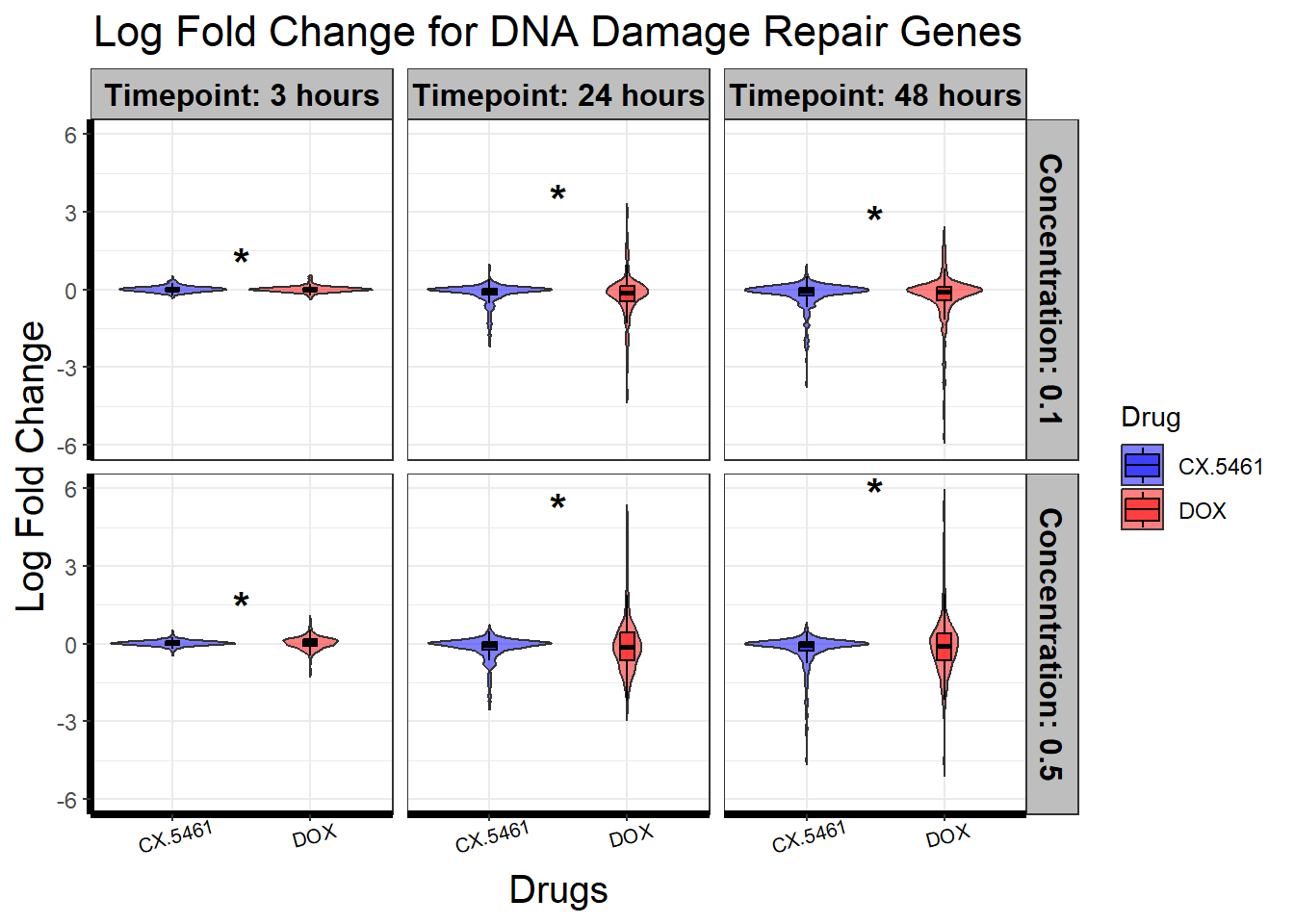
📌 DNA Damage Repair logFC distribution
# Load necessary libraries
library(dplyr)
library(ggplot2)
library(tidyr)
library(org.Hs.eg.db)
library(car)  # For Levene's Test
Warning: package 'car' was built under R version 4.3.3Warning: package 'carData' was built under R version 4.3.1# Read DNA Damage Response Gene List
DNA_damage <- read.csv("data/DNA_Damage.csv", stringsAsFactors = FALSE)
# Convert gene symbols to Entrez IDs
DNA_damage <- DNA_damage %>%
mutate(Entrez_ID = mapIds(org.Hs.eg.db,
keys = Symbol,
column = "ENTREZID",
keytype = "SYMBOL",
multiVals = "first"))
DNA_damage_genes <- na.omit(DNA_damage$Entrez_ID)
all_toptables <- bind_rows(
CX_0.1_3 %>% mutate(Drug = "CX.5461", Concentration = 0.1, Timepoint = "3"),
CX_0.1_24 %>% mutate(Drug = "CX.5461", Concentration = 0.1, Timepoint = "24"),
CX_0.1_48 %>% mutate(Drug = "CX.5461", Concentration = 0.1, Timepoint = "48"),
CX_0.5_3 %>% mutate(Drug = "CX.5461", Concentration = 0.5, Timepoint = "3"),
CX_0.5_24 %>% mutate(Drug = "CX.5461", Concentration = 0.5, Timepoint = "24"),
CX_0.5_48 %>% mutate(Drug = "CX.5461", Concentration = 0.5, Timepoint = "48"),
DOX_0.1_3 %>% mutate(Drug = "DOX", Concentration = 0.1, Timepoint = "3"),
DOX_0.1_24 %>% mutate(Drug = "DOX", Concentration = 0.1, Timepoint = "24"),
DOX_0.1_48 %>% mutate(Drug = "DOX", Concentration = 0.1, Timepoint = "48"),
DOX_0.5_3 %>% mutate(Drug = "DOX", Concentration = 0.5, Timepoint = "3"),
DOX_0.5_24 %>% mutate(Drug = "DOX", Concentration = 0.5, Timepoint = "24"),
DOX_0.5_48 %>% mutate(Drug = "DOX", Concentration = 0.5, Timepoint = "48")
)
filtered_toptables <- all_toptables %>%
filter(Entrez_ID %in% DNA_damage_genes)
filtered_toptables <- filtered_toptables %>%
mutate(
Drug = factor(Drug, levels = c("CX.5461", "DOX")), # CX first
Timepoint = factor(Timepoint, levels = c("3", "24", "48"),
labels = c("Timepoint: 3 hours", "Timepoint: 24 hours", "Timepoint: 48 hours")),
Concentration = factor(Concentration, levels = c(0.1, 0.5),
labels = c("Concentration: 0.1", "Concentration: 0.5"))
)
levene_results <- filtered_toptables %>%
group_by(Timepoint, Concentration) %>%
summarise(p_value = leveneTest(logFC ~ Drug, data = .)$`Pr(>F)`[1], .groups = "drop") %>%
mutate(significance = ifelse(p_value < 0.05, "*", "")) # Use p < 0.05 threshold for stars
# **🔹 Determine Y-axis position for Stars**
star_positions <- filtered_toptables %>%
group_by(Timepoint, Concentration, Drug) %>%
summarise(y_pos = max(logFC, na.rm = TRUE) + 0.5, .groups = "drop") %>%
group_by(Timepoint, Concentration) %>%
summarise(y_pos = max(y_pos), .groups = "drop")
# **🔹 Merge Levene test results with Y positions**
levene_results_plot <- levene_results %>%
left_join(star_positions, by = c("Timepoint", "Concentration")) %>%
mutate(x_position = 1.5) # Centered between CX & DOX
ggplot(filtered_toptables, aes(x = Drug, y = logFC, fill = Drug)) +
geom_violin(trim = FALSE, alpha = 0.5) + # Violin plot for logFC
geom_boxplot(width = 0.1, outlier.shape = NA, color = "black", alpha = 0.5) + # Add boxplot inside violin
scale_fill_manual(values = c("CX.5461" = "blue", "DOX" = "red")) +
facet_grid(Concentration ~ Timepoint) +
geom_text(
data = levene_results_plot %>% filter(significance == "*"), # Only plot significant comparisons
aes(x = x_position, y = y_pos, label = significance),
size = 6, fontface = "bold", color = "black", inherit.aes = FALSE
) +
theme_bw() +
xlab("Drugs") +
ylab("Log Fold Change") +
ggtitle("Log Fold Change for DNA Damage Repair Genes") +
theme(
plot.title = element_text(size = rel(1.5), hjust = 0.5),
axis.title = element_text(size = 15, color = "black"),
axis.line = element_line(linewidth = 1.5),
strip.background = element_rect(fill = "gray"),
strip.text = element_text(size = 12, color = "black", face = "bold"),
axis.text.x = element_text(size = 8, color = "black", angle = 15)
)
📌 Generate Boxplots for DNA Damage Repair Genes
for (gene in dna_repair_genes) {
  data_info <- process_gene_data(gene)
  p <- ggplot(data_info$long_data, aes(x = Condition, y = log2CPM, fill = Drug)) +
    geom_boxplot(outlier.shape = NA) +
    scale_fill_manual(values = c("CX" = "#0000FF", "DOX" = "#e6d800", "VEH" = "#FF00FF")) +
    geom_point(aes(color = Indv), size = 2, alpha = 0.5, position = position_jitter(width = 0.2, height = 0)) +
    geom_text(data = data_info$significance_labels, aes(x = Condition, y = max_log2CPM + 0.5, label = Significance),
              inherit.aes = FALSE, size = 6, color = "black") +
    ggtitle(paste("Log2CPM Expression of", gene)) +
    labs(x = "Treatment", y = "log2CPM") +
    theme_bw() +
    theme(plot.title = element_text(size = rel(2), hjust = 0.5),
          axis.title = element_text(size = 15, color = "black"),
          axis.text.x = element_text(size = 10, color = "black", angle = 90, hjust = 1))

  print(p)
}
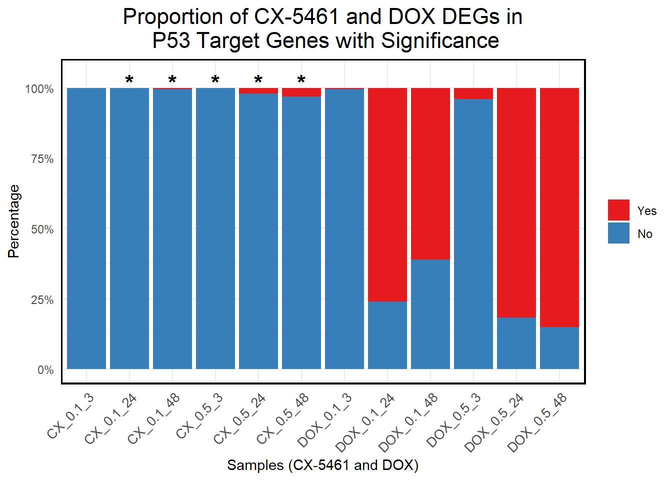
📌 P53 target genes Proportion
📌 P53 target genes Proportion with Chi-Square Test
# Load necessary libraries
library(dplyr)
library(ggplot2)
library(tidyr)
library(org.Hs.eg.db)

# Read P53 Target Genes List
P53_Target <- read.csv("data/P53_Target.csv", stringsAsFactors = FALSE)

# Convert gene symbols to Entrez IDs
P53_Target <- P53_Target %>%
  mutate(Entrez_ID = mapIds(org.Hs.eg.db,
                            keys = Symbol,
                            column = "ENTREZID",
                            keytype = "SYMBOL",
                            multiVals = "first"))

# Extract valid Entrez_IDs
P53_Target_genes <- na.omit(P53_Target$Entrez_ID)
total_P53_Target_genes <- length(P53_Target_genes)  # Total number of P53 target genes

# Function to calculate the presence of P53 target genes in DEGs
calculate_proportion <- function(deg_list, drug_name) {
  data.frame(
    Sample = names(deg_list),
    Drug = drug_name,
    P53_Target_DEGs = sapply(deg_list, function(ids) sum(ids %in% P53_Target_genes)),  # DEGs present in P53 target set
    Non_P53_Target_DEGs = sapply(deg_list, function(ids) total_P53_Target_genes - sum(ids %in% P53_Target_genes))  # Remaining P53 target genes
  ) %>%
    mutate(
      Yes_Proportion = (P53_Target_DEGs / total_P53_Target_genes) * 100,  # Percentage of DEGs in P53 target genes
      No_Proportion = (Non_P53_Target_DEGs / total_P53_Target_genes) * 100  # Remaining P53 target genes as No
    )
}

# Define CX-5461 and DOX DEG lists
CX_DEGs <- list(
  "CX_0.1_3" = DEG1, "CX_0.1_24" = DEG2, "CX_0.1_48" = DEG3,
  "CX_0.5_3" = DEG4, "CX_0.5_24" = DEG5, "CX_0.5_48" = DEG6
)

DOX_DEGs <- list(
  "DOX_0.1_3" = DEG7, "DOX_0.1_24" = DEG8, "DOX_0.1_48" = DEG9,
  "DOX_0.5_3" = DEG10, "DOX_0.5_24" = DEG11, "DOX_0.5_48" = DEG12
)

# Calculate proportions for CX-5461 and DOX
CX_proportion <- calculate_proportion(CX_DEGs, "CX-5461")
DOX_proportion <- calculate_proportion(DOX_DEGs, "DOX")

# Combine data
proportion_data <- bind_rows(CX_proportion, DOX_proportion)

# Convert to long format for stacked bar plot
proportion_long <- proportion_data %>%
  select(Sample, Drug, Yes_Proportion, No_Proportion) %>%
  pivot_longer(cols = c(Yes_Proportion, No_Proportion), names_to = "Category", values_to = "Percentage") %>%
  mutate(Category = ifelse(Category == "Yes_Proportion", "Yes", "No"))

# **Ensure correct order of samples on X-axis**
sample_order <- c(
  "CX_0.1_3", "CX_0.1_24", "CX_0.1_48", "CX_0.5_3", "CX_0.5_24", "CX_0.5_48",
  "DOX_0.1_3", "DOX_0.1_24", "DOX_0.1_48", "DOX_0.5_3", "DOX_0.5_24", "DOX_0.5_48"
)
proportion_long$Sample <- factor(proportion_long$Sample, levels = sample_order, ordered = TRUE)

# **Ensure "Yes" is on top and "No" is at the bottom in stacked bars**
proportion_long$Category <- factor(proportion_long$Category, levels = c("Yes", "No"))

# **Perform Chi-Square Test for CX vs DOX at each timepoint**
chi_square_results <- data.frame(Sample = character(), P_Value = numeric())

for (i in seq(1, 6)) {  # Pairwise comparison (CX vs DOX)
  cx_sample <- sample_order[i]
  dox_sample <- sample_order[i + 6]  # Matches CX_0.1_3 with DOX_0.1_3, etc.

  cx_data <- filter(proportion_data, Sample == cx_sample)
  dox_data <- filter(proportion_data, Sample == dox_sample)

  # Construct contingency table for Chi-Square test
  contingency_table <- matrix(
    c(cx_data$P53_Target_DEGs, cx_data$Non_P53_Target_DEGs,
      dox_data$P53_Target_DEGs, dox_data$Non_P53_Target_DEGs),
    nrow = 2, byrow = TRUE
  )

  # Run Chi-Square Test
  test_result <- chisq.test(contingency_table)
  p_value <- test_result$p.value

  # Store results
  chi_square_results <- rbind(chi_square_results, data.frame(Sample = cx_sample, P_Value = p_value))
}

# Add significance stars
chi_square_results$Significant <- ifelse(chi_square_results$P_Value < 0.05, "*", "")

# Merge Chi-Square results
proportion_long <- left_join(proportion_long, chi_square_results, by = "Sample")

# **Save output**
write.csv(proportion_long, "C:/Work/Postdoc_UTMB/CX-5461 Project/Transcriptome literatures/lit2/Proportion_Stacked_P53_Target_DEGs_with_ChiSquare.csv", row.names = FALSE)

# Define correct factor orders for samples
sample_order <- c(
  "CX_0.1_3", "CX_0.1_24", "CX_0.1_48", "CX_0.5_3", "CX_0.5_24", "CX_0.5_48",
  "DOX_0.1_3", "DOX_0.1_24", "DOX_0.1_48", "DOX_0.5_3", "DOX_0.5_24", "DOX_0.5_48"
)

# Reapply factor levels for correct order in both proportion_data and proportion_long
proportion_data$Sample <- factor(proportion_data$Sample, levels = sample_order, ordered = TRUE)
proportion_long$Sample <- factor(proportion_long$Sample, levels = sample_order, ordered = TRUE)

# **Fix: Ensure "Yes" is on top and "No" is at the bottom in stacked bars**
proportion_long$Category <- factor(proportion_long$Category, levels = c("Yes", "No"))


# **Generate Stacked Bar Plot with Correct X-Axis Order**
ggplot(proportion_long, aes(x = Sample, y = Percentage, fill = Category)) +
  geom_bar(stat = "identity", position = "stack") +  # Stacked bars
  geom_text(data = subset(proportion_long, Significant == "*"),
            aes(x = Sample, y = 102, label = "*"),  # Position stars slightly above 100%
            size = 6, color = "black", fontface = "bold") +
  scale_y_continuous(labels = scales::percent_format(scale = 1), limits = c(0, 105)) +  # Increase Y-axis slightly
  scale_fill_manual(values = c("Yes" = "#e41a1c", "No" = "#377eb8")) +  # Yes (Red), No (Blue)
  labs(
    title = "Proportion of CX-5461 and DOX DEGs in\n P53 Target Genes with Significance",
    x = "Samples (CX-5461 and DOX)",
    y = "Percentage",
    fill = "Category"
  ) +
  theme_minimal() +
  theme(
    plot.title = element_text(size = rel(1.5), hjust = 0.5),
    axis.text.x = element_text(size = 10, angle = 45, hjust = 1),
    legend.title = element_blank(),
    panel.border = element_rect(color = "black", fill = NA, linewidth = 1.2),
    strip.background = element_blank(),
    strip.text = element_text(size = 12, face = "bold")
  )
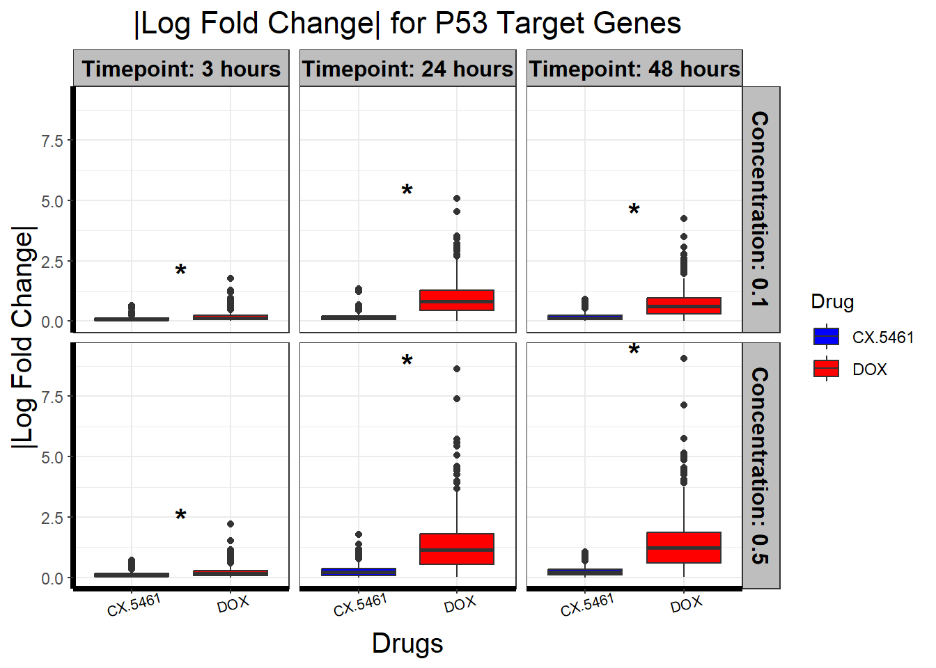
📌 P53 target genes abs logFC distribution
# Load necessary libraries
library(dplyr)
library(ggplot2)
library(tidyr)
library(org.Hs.eg.db)
library(rstatix)

# **🔹 Read P53 Target Genes List**
P53_Target <- read.csv("data/P53_Target.csv", stringsAsFactors = FALSE)

# **🔹 Convert gene symbols to Entrez IDs**
P53_Target <- P53_Target %>%
  mutate(Entrez_ID = mapIds(org.Hs.eg.db,
                            keys = Symbol,
                            column = "ENTREZID",
                            keytype = "SYMBOL",
                            multiVals = "first"))

P53_Target_genes <- na.omit(P53_Target$Entrez_ID)

# **🔹 Combine all subset_toptables into a single data frame with metadata**
all_toptables <- bind_rows(
  CX_0.1_3 %>% mutate(Drug = "CX.5461", Concentration = 0.1, Timepoint = "3"),
  CX_0.1_24 %>% mutate(Drug = "CX.5461", Concentration = 0.1, Timepoint = "24"),
  CX_0.1_48 %>% mutate(Drug = "CX.5461", Concentration = 0.1, Timepoint = "48"),
  CX_0.5_3 %>% mutate(Drug = "CX.5461", Concentration = 0.5, Timepoint = "3"),
  CX_0.5_24 %>% mutate(Drug = "CX.5461", Concentration = 0.5, Timepoint = "24"),
  CX_0.5_48 %>% mutate(Drug = "CX.5461", Concentration = 0.5, Timepoint = "48"),
  DOX_0.1_3 %>% mutate(Drug = "DOX", Concentration = 0.1, Timepoint = "3"),
  DOX_0.1_24 %>% mutate(Drug = "DOX", Concentration = 0.1, Timepoint = "24"),
  DOX_0.1_48 %>% mutate(Drug = "DOX", Concentration = 0.1, Timepoint = "48"),
  DOX_0.5_3 %>% mutate(Drug = "DOX", Concentration = 0.5, Timepoint = "3"),
  DOX_0.5_24 %>% mutate(Drug = "DOX", Concentration = 0.5, Timepoint = "24"),
  DOX_0.5_48 %>% mutate(Drug = "DOX", Concentration = 0.5, Timepoint = "48")
)

# **🔹 Filter data for P53 Target Genes**
filtered_toptables <- all_toptables %>%
  filter(Entrez_ID %in% P53_Target_genes) %>%
  mutate(abs_logFC = abs(logFC))  # Compute absolute logFC

# **🔹 Ensure correct ordering of Timepoints & Concentrations**
filtered_toptables <- filtered_toptables %>%
  mutate(
    Drug = factor(Drug, levels = c("CX.5461", "DOX")),  # CX first
    Timepoint = factor(Timepoint, levels = c("3", "24", "48"),
                       labels = c("Timepoint: 3 hours", "Timepoint: 24 hours", "Timepoint: 48 hours")),
    Concentration = factor(Concentration, levels = c(0.1, 0.5),
                           labels = c("Concentration: 0.1", "Concentration: 0.5"))
  )

# **🔹 Wilcoxon Test for CX vs DOX**
wilcox_results <- filtered_toptables %>%
  group_by(Timepoint, Concentration) %>%
  wilcox_test(abs_logFC ~ Drug) %>%
  adjust_pvalue(method = "bonferroni") %>%
  mutate(significance = ifelse(p < 0.05, "*", ""))  # Assign stars if p < 0.05

# **🔹 Determine Y-axis position for Stars**
star_positions <- filtered_toptables %>%
  group_by(Timepoint, Concentration, Drug) %>%
  summarise(y_pos = max(abs_logFC, na.rm = TRUE) + 0.2, .groups = "drop") %>%
  group_by(Timepoint, Concentration) %>%
  summarise(y_pos = max(y_pos), .groups = "drop")

# **🔹 Merge Wilcoxon Test results with Star Positions**
wilcox_results_plot <- wilcox_results %>%
  left_join(star_positions, by = c("Timepoint", "Concentration")) %>%
  mutate(x_position = 1.5)  # Place stars in the middle between CX & DOX

# **🔹 Generate Boxplot for LogFC of P53 Target Genes**
ggplot(filtered_toptables, aes(x = Drug, y = abs_logFC, fill = Drug)) +
  geom_boxplot() +
  scale_fill_manual(values = c("CX.5461" = "blue", "DOX" = "red")) +
  facet_grid(Concentration ~ Timepoint) +
  geom_text(
    data = wilcox_results_plot,
    aes(x = x_position, y = y_pos, label = significance),
    size = 6, fontface = "bold", color = "black", inherit.aes = FALSE
  ) +
  theme_bw() +
  xlab("Drugs") +
  ylab("|Log Fold Change|") +
  ggtitle("|Log Fold Change| for P53 Target Genes") +
  theme(
    plot.title = element_text(size = rel(1.5), hjust = 0.5),
    axis.title = element_text(size = 15, color = "black"),
    axis.line = element_line(linewidth = 1.5),
    strip.background = element_rect(fill = "gray"),
    strip.text = element_text(size = 12, color = "black", face = "bold"),
    axis.text.x = element_text(size = 8, color = "black", angle = 15)
  )
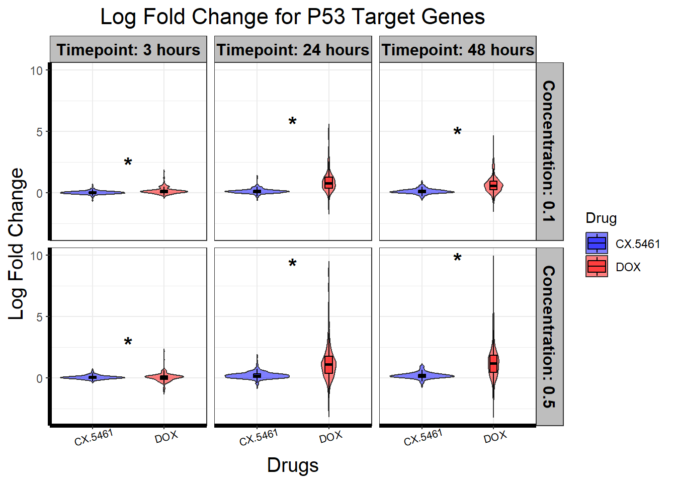
📌 P53 Target Genes logFC distribution
# Load necessary libraries
library(dplyr)
library(ggplot2)
library(tidyr)
library(org.Hs.eg.db)
library(car)  # For Levene's Test

# Read P53 Target Genes List
P53_Target <- read.csv("data/P53_Target.csv", stringsAsFactors = FALSE)

# Convert gene symbols to Entrez IDs
P53_Target <- P53_Target %>%
  mutate(Entrez_ID = mapIds(org.Hs.eg.db,
                            keys = Symbol,
                            column = "ENTREZID",
                            keytype = "SYMBOL",
                            multiVals = "first"))

P53_Target_genes <- na.omit(P53_Target$Entrez_ID)

# **🔹 Combine all subset_toptables into a single data frame with metadata**
all_toptables <- bind_rows(
  CX_0.1_3 %>% mutate(Drug = "CX.5461", Concentration = 0.1, Timepoint = "3"),
  CX_0.1_24 %>% mutate(Drug = "CX.5461", Concentration = 0.1, Timepoint = "24"),
  CX_0.1_48 %>% mutate(Drug = "CX.5461", Concentration = 0.1, Timepoint = "48"),
  CX_0.5_3 %>% mutate(Drug = "CX.5461", Concentration = 0.5, Timepoint = "3"),
  CX_0.5_24 %>% mutate(Drug = "CX.5461", Concentration = 0.5, Timepoint = "24"),
  CX_0.5_48 %>% mutate(Drug = "CX.5461", Concentration = 0.5, Timepoint = "48"),
  DOX_0.1_3 %>% mutate(Drug = "DOX", Concentration = 0.1, Timepoint = "3"),
  DOX_0.1_24 %>% mutate(Drug = "DOX", Concentration = 0.1, Timepoint = "24"),
  DOX_0.1_48 %>% mutate(Drug = "DOX", Concentration = 0.1, Timepoint = "48"),
  DOX_0.5_3 %>% mutate(Drug = "DOX", Concentration = 0.5, Timepoint = "3"),
  DOX_0.5_24 %>% mutate(Drug = "DOX", Concentration = 0.5, Timepoint = "24"),
  DOX_0.5_48 %>% mutate(Drug = "DOX", Concentration = 0.5, Timepoint = "48")
)

# **🔹 Filter data for P53 target genes**
filtered_toptables <- all_toptables %>%
  filter(Entrez_ID %in% P53_Target_genes)

# **🔹 Factorize variables for ordered plotting**
filtered_toptables <- filtered_toptables %>%
  mutate(
    Drug = factor(Drug, levels = c("CX.5461", "DOX")),  # CX first
    Timepoint = factor(Timepoint, levels = c("3", "24", "48"),
                       labels = c("Timepoint: 3 hours", "Timepoint: 24 hours", "Timepoint: 48 hours")),
    Concentration = factor(Concentration, levels = c(0.1, 0.5),
                           labels = c("Concentration: 0.1", "Concentration: 0.5"))
  )

# **🔹 Perform Levene's test for variability differences**
levene_results <- filtered_toptables %>%
  group_by(Timepoint, Concentration) %>%
  summarise(p_value = leveneTest(logFC ~ Drug, data = .)$`Pr(>F)`[1], .groups = "drop") %>%
  mutate(significance = ifelse(p_value < 0.05, "*", ""))  # Use p < 0.05 threshold for stars

# **🔹 Determine Y-axis position for Stars**
star_positions <- filtered_toptables %>%
  group_by(Timepoint, Concentration, Drug) %>%
  summarise(y_pos = max(logFC, na.rm = TRUE) + 0.5, .groups = "drop") %>%
  group_by(Timepoint, Concentration) %>%
  summarise(y_pos = max(y_pos), .groups = "drop")

# **🔹 Merge Levene test results with Y positions**
levene_results_plot <- levene_results %>%
  left_join(star_positions, by = c("Timepoint", "Concentration")) %>%
  mutate(x_position = 1.5)  # Centered between CX & DOX

# **🔹 Generate Violin Plot with Boxplot & Significance Stars**
ggplot(filtered_toptables, aes(x = Drug, y = logFC, fill = Drug)) +
  geom_violin(trim = FALSE, alpha = 0.5) +  # Violin plot for logFC
  geom_boxplot(width = 0.1, outlier.shape = NA, color = "black", alpha = 0.5) +  # Add boxplot inside violin
  scale_fill_manual(values = c("CX.5461" = "blue", "DOX" = "red")) +
  facet_grid(Concentration ~ Timepoint) +
  geom_text(
    data = levene_results_plot %>% filter(significance == "*"),  # Only plot significant comparisons
    aes(x = x_position, y = y_pos, label = significance),
    size = 6, fontface = "bold", color = "black", inherit.aes = FALSE
  ) +
  theme_bw() +
  xlab("Drugs") +
  ylab("Log Fold Change") +
  ggtitle("Log Fold Change for P53 Target Genes") +
  theme(
    plot.title = element_text(size = rel(1.5), hjust = 0.5),
    axis.title = element_text(size = 15, color = "black"),
    axis.line = element_line(linewidth = 1.5),
    strip.background = element_rect(fill = "gray"),
    strip.text = element_text(size = 12, color = "black", face = "bold"),
    axis.text.x = element_text(size = 8, color = "black", angle = 15)
  )
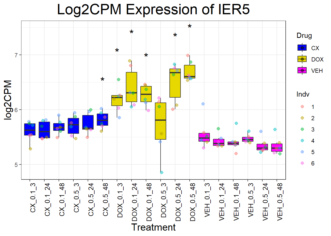
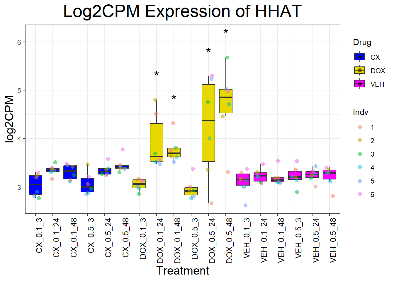
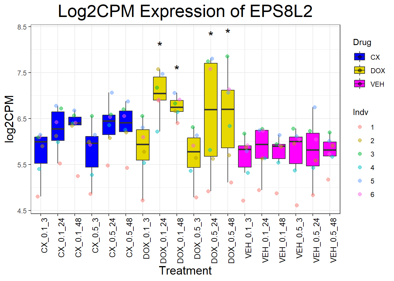
📌 Generate Boxplots for P53 Target Genes
for (gene in p53_target_genes) {
  data_info <- process_gene_data(gene)
  p <- ggplot(data_info$long_data, aes(x = Condition, y = log2CPM, fill = Drug)) +
    geom_boxplot(outlier.shape = NA) +
    scale_fill_manual(values = c("CX" = "#0000FF", "DOX" = "#e6d800", "VEH" = "#FF00FF")) +
    geom_point(aes(color = Indv), size = 2, alpha = 0.5, position = position_jitter(width = 0.2, height = 0)) +
    geom_text(data = data_info$significance_labels, aes(x = Condition, y = max_log2CPM + 0.5, label = Significance),
              inherit.aes = FALSE, size = 6, color = "black") +
    ggtitle(paste("Log2CPM Expression of", gene)) +
    labs(x = "Treatment", y = "log2CPM") +
    theme_bw() +
    theme(plot.title = element_text(size = rel(2), hjust = 0.5),
          axis.title = element_text(size = 15, color = "black"),
          axis.text.x = element_text(size = 10, color = "black", angle = 90, hjust = 1))

  print(p)
}
sessionInfo()R version 4.3.0 (2023-04-21 ucrt)
Platform: x86_64-w64-mingw32/x64 (64-bit)
Running under: Windows 11 x64 (build 26100)
Matrix products: default
locale:
[1] LC_COLLATE=English_United States.utf8
[2] LC_CTYPE=English_United States.utf8
[3] LC_MONETARY=English_United States.utf8
[4] LC_NUMERIC=C
[5] LC_TIME=English_United States.utf8
time zone: America/Chicago
tzcode source: internal
attached base packages:
[1] stats4 stats graphics grDevices utils datasets methods
[8] base
other attached packages:
[1] car_3.1-3 carData_3.0-5 rstatix_0.7.2
[4] clusterProfiler_4.10.1 org.Hs.eg.db_3.18.0 AnnotationDbi_1.64.1
[7] IRanges_2.36.0 S4Vectors_0.40.2 Biobase_2.62.0
[10] BiocGenerics_0.48.1 tidyr_1.3.1 dplyr_1.1.4
[13] ggplot2_3.5.2
loaded via a namespace (and not attached):
[1] RColorBrewer_1.1-3 rstudioapi_0.17.1 jsonlite_2.0.0
[4] magrittr_2.0.3 farver_2.1.2 rmarkdown_2.29
[7] fs_1.6.3 zlibbioc_1.48.2 vctrs_0.6.5
[10] memoise_2.0.1 RCurl_1.98-1.17 ggtree_3.10.1
[13] htmltools_0.5.8.1 broom_1.0.8 Formula_1.2-5
[16] gridGraphics_0.5-1 sass_0.4.10 bslib_0.9.0
[19] plyr_1.8.9 cachem_1.1.0 whisker_0.4.1
[22] igraph_2.1.4 lifecycle_1.0.4 pkgconfig_2.0.3
[25] Matrix_1.6-1.1 R6_2.6.1 fastmap_1.2.0
[28] gson_0.1.0 GenomeInfoDbData_1.2.11 digest_0.6.34
[31] aplot_0.2.5 enrichplot_1.22.0 colorspace_2.1-0
[34] patchwork_1.3.0 rprojroot_2.0.4 RSQLite_2.3.9
[37] labeling_0.4.3 httr_1.4.7 polyclip_1.10-7
[40] abind_1.4-8 compiler_4.3.0 bit64_4.6.0-1
[43] withr_3.0.2 backports_1.5.0 BiocParallel_1.36.0
[46] viridis_0.6.5 DBI_1.2.3 ggforce_0.4.2
[49] MASS_7.3-60 HDO.db_0.99.1 tools_4.3.0
[52] ape_5.8-1 scatterpie_0.2.4 httpuv_1.6.15
[55] glue_1.7.0 nlme_3.1-168 GOSemSim_2.28.1
[58] promises_1.3.2 grid_4.3.0 shadowtext_0.1.4
[61] reshape2_1.4.4 fgsea_1.28.0 generics_0.1.3
[64] gtable_0.3.6 data.table_1.17.0 tidygraph_1.3.1
[67] XVector_0.42.0 ggrepel_0.9.6 pillar_1.10.2
[70] stringr_1.5.1 yulab.utils_0.2.0 later_1.3.2
[73] splines_4.3.0 tweenr_2.0.3 treeio_1.26.0
[76] lattice_0.22-7 bit_4.6.0 tidyselect_1.2.1
[79] GO.db_3.18.0 Biostrings_2.70.3 knitr_1.50
[82] git2r_0.36.2 gridExtra_2.3 xfun_0.52
[85] graphlayouts_1.2.2 stringi_1.8.3 workflowr_1.7.1
[88] lazyeval_0.2.2 ggfun_0.1.8 yaml_2.3.10
[91] evaluate_1.0.3 codetools_0.2-20 ggraph_2.2.1
[94] tibble_3.2.1 qvalue_2.34.0 ggplotify_0.1.2
[97] cli_3.6.1 munsell_0.5.1 jquerylib_0.1.4
[100] Rcpp_1.0.12 GenomeInfoDb_1.38.8 png_0.1-8
[103] parallel_4.3.0 blob_1.2.4 DOSE_3.28.2
[106] bitops_1.0-9 viridisLite_0.4.2 tidytree_0.4.6
[109] scales_1.3.0 purrr_1.0.4 crayon_1.5.3
[112] rlang_1.1.3 cowplot_1.1.3 fastmatch_1.1-6
[115] KEGGREST_1.42.0