Correlation between CX and DOX logFC
Last updated: 2025-03-30
Checks: 7 0
Knit directory: CX5461_Project/
This reproducible R Markdown analysis was created with workflowr (version 1.7.1). The Checks tab describes the reproducibility checks that were applied when the results were created. The Past versions tab lists the development history.
Great! Since the R Markdown file has been committed to the Git repository, you know the exact version of the code that produced these results.
Great job! The global environment was empty. Objects defined in the global environment can affect the analysis in your R Markdown file in unknown ways. For reproduciblity it’s best to always run the code in an empty environment.
The command set.seed(20250129) was run prior to running
the code in the R Markdown file. Setting a seed ensures that any results
that rely on randomness, e.g. subsampling or permutations, are
reproducible.
Great job! Recording the operating system, R version, and package versions is critical for reproducibility.
Nice! There were no cached chunks for this analysis, so you can be confident that you successfully produced the results during this run.
Great job! Using relative paths to the files within your workflowr project makes it easier to run your code on other machines.
Great! You are using Git for version control. Tracking code development and connecting the code version to the results is critical for reproducibility.
The results in this page were generated with repository version 2f71a7f. See the Past versions tab to see a history of the changes made to the R Markdown and HTML files.
Note that you need to be careful to ensure that all relevant files for
the analysis have been committed to Git prior to generating the results
(you can use wflow_publish or
wflow_git_commit). workflowr only checks the R Markdown
file, but you know if there are other scripts or data files that it
depends on. Below is the status of the Git repository when the results
were generated:
Ignored files:
    Ignored:    .RData
    Ignored:    .Rhistory
    Ignored:    .Rproj.user/

Untracked files:
    Untracked:  0.1 box.svg
    Untracked:  0.1 density.svg
    Untracked:  0.1.emf
    Untracked:  0.1.svg
    Untracked:  0.5 box.svg
    Untracked:  0.5 density.svg
    Untracked:  0.5.svg
    Untracked:  Rplot.svg
    Untracked:  Rplot01.svg
    Untracked:  Rplot02.svg
    Untracked:  Rplot03.svg
Note that any generated files, e.g. HTML, png, CSS, etc., are not included in this status report because it is ok for generated content to have uncommitted changes.
These are the previous versions of the repository in which changes were
made to the R Markdown (analysis/CX_DOX.Rmd) and HTML
(docs/CX_DOX.html) files. If you’ve configured a remote Git
repository (see ?wflow_git_remote), click on the hyperlinks
in the table below to view the files as they were in that past version.
| File | Version | Author | Date | Message |
|---|---|---|---|---|
| html | 2f71a7f | sayanpaul01 | 2025-03-30 | Commit |
| Rmd | 7f99e68 | sayanpaul01 | 2025-03-30 | Commit |
| html | 7f99e68 | sayanpaul01 | 2025-03-30 | Commit |
| Rmd | 61329df | sayanpaul01 | 2025-03-16 | Commit |
| html | 61329df | sayanpaul01 | 2025-03-16 | Commit |
| Rmd | aec1deb | sayanpaul01 | 2025-03-02 | Commit |
| html | aec1deb | sayanpaul01 | 2025-03-02 | Commit |
📌 Correlation between CX and DOX logFC
📌 Load Required Libraries
# Load necessary libraries
library(dplyr)
Warning: package 'dplyr' was built under R version 4.3.2library(ggplot2)Warning: package 'ggplot2' was built under R version 4.3.3📌 Correlation Scatter plot
# Load DEGs Data
CX_0.1_3 <- read.csv("data/DEGs/Toptable_CX_0.1_3.csv")
CX_0.1_24 <- read.csv("data/DEGs/Toptable_CX_0.1_24.csv")
CX_0.1_48 <- read.csv("data/DEGs/Toptable_CX_0.1_48.csv")
CX_0.5_3 <- read.csv("data/DEGs/Toptable_CX_0.5_3.csv")
CX_0.5_24 <- read.csv("data/DEGs/Toptable_CX_0.5_24.csv")
CX_0.5_48 <- read.csv("data/DEGs/Toptable_CX_0.5_48.csv")

DOX_0.1_3 <- read.csv("data/DEGs/Toptable_DOX_0.1_3.csv")
DOX_0.1_24 <- read.csv("data/DEGs/Toptable_DOX_0.1_24.csv")
DOX_0.1_48 <- read.csv("data/DEGs/Toptable_DOX_0.1_48.csv")
DOX_0.5_3 <- read.csv("data/DEGs/Toptable_DOX_0.5_3.csv")
DOX_0.5_24 <- read.csv("data/DEGs/Toptable_DOX_0.5_24.csv")
DOX_0.5_48 <- read.csv("data/DEGs/Toptable_DOX_0.5_48.csv")

# Extract Significant DEGs
DEG1 <- as.character(CX_0.1_3$Entrez_ID[CX_0.1_3$adj.P.Val < 0.05])
DEG2 <- as.character(CX_0.1_24$Entrez_ID[CX_0.1_24$adj.P.Val < 0.05])
DEG3 <- as.character(CX_0.1_48$Entrez_ID[CX_0.1_48$adj.P.Val < 0.05])
DEG4 <- as.character(CX_0.5_3$Entrez_ID[CX_0.5_3$adj.P.Val < 0.05])
DEG5 <- as.character(CX_0.5_24$Entrez_ID[CX_0.5_24$adj.P.Val < 0.05])
DEG6 <- as.character(CX_0.5_48$Entrez_ID[CX_0.5_48$adj.P.Val < 0.05])
DEG7 <- as.character(DOX_0.1_3$Entrez_ID[DOX_0.1_3$adj.P.Val < 0.05])
DEG8 <- as.character(DOX_0.1_24$Entrez_ID[DOX_0.1_24$adj.P.Val < 0.05])
DEG9 <- as.character(DOX_0.1_48$Entrez_ID[DOX_0.1_48$adj.P.Val < 0.05])
DEG10 <- as.character(DOX_0.5_3$Entrez_ID[DOX_0.5_3$adj.P.Val < 0.05])
DEG11 <- as.character(DOX_0.5_24$Entrez_ID[DOX_0.5_24$adj.P.Val < 0.05])
DEG12 <- as.character(DOX_0.5_48$Entrez_ID[DOX_0.5_48$adj.P.Val < 0.05])

# Ensure Entrez_ID is a character across all datasets
datasets <- list(CX_0.1_3, CX_0.1_24, CX_0.1_48, CX_0.5_3, CX_0.5_24, CX_0.5_48,
                 DOX_0.1_3, DOX_0.1_24, DOX_0.1_48, DOX_0.5_3, DOX_0.5_24, DOX_0.5_48)

for (i in seq_along(datasets)) {
  datasets[[i]]$Entrez_ID <- as.character(datasets[[i]]$Entrez_ID)
}

# Define dataset pairs for correlation analysis
dataset_pairs <- list(
  list("CX_0.1_3", CX_0.1_3, "DOX_0.1_3", DOX_0.1_3, "3 hours", "0.1 micromolar"),
  list("CX_0.1_24", CX_0.1_24, "DOX_0.1_24", DOX_0.1_24, "24 hours", "0.1 micromolar"),
  list("CX_0.1_48", CX_0.1_48, "DOX_0.1_48", DOX_0.1_48, "48 hours", "0.1 micromolar"),
  list("CX_0.5_3", CX_0.5_3, "DOX_0.5_3", DOX_0.5_3, "3 hours", "0.5 micromolar"),
  list("CX_0.5_24", CX_0.5_24, "DOX_0.5_24", DOX_0.5_24, "24 hours", "0.5 micromolar"),
  list("CX_0.5_48", CX_0.5_48, "DOX_0.5_48", DOX_0.5_48, "48 hours", "0.5 micromolar")
)

# Create an empty list to store merged data
merged_data_list <- list()

# Loop through dataset pairs and merge based on Entrez_ID
for (pair in dataset_pairs) {
  cx_name <- pair[[1]]
  cx_data <- pair[[2]]
  dox_name <- pair[[3]]
  dox_data <- pair[[4]]
  timepoint <- pair[[5]]
  concentration <- pair[[6]]

  merged_data <- merge(cx_data, dox_data, by = "Entrez_ID", suffixes = c("_CX", "_DOX"))
  merged_data$Timepoint <- timepoint
  merged_data$Concentration <- concentration

  merged_data_list[[paste(cx_name, dox_name, sep = "_vs_")]] <- merged_data
}

# Combine all merged datasets into a single dataframe
combined_data <- do.call(rbind, merged_data_list)

# Select necessary columns and rename them
combined_data <- combined_data %>%
  dplyr::select(Entrez_ID, logFC_CX = logFC_CX, logFC_DOX = logFC_DOX, Timepoint, Concentration)

# Ensure timepoints and concentrations are in the correct order
combined_data$Timepoint <- factor(combined_data$Timepoint, levels = c("3 hours", "24 hours", "48 hours"))
combined_data$Concentration <- factor(combined_data$Concentration, levels = c("0.1 micromolar", "0.5 micromolar"))

# **Step 1: Compute global min and max for y-axis scale**
y_min <- min(combined_data$logFC_DOX, na.rm = TRUE)
y_max <- max(combined_data$logFC_DOX, na.rm = TRUE)

# **Step 2: Compute correlations for each dataset with exact p-values**
correlations <- combined_data %>%
  group_by(Concentration, Timepoint) %>%
  summarise(
    r_value = cor(logFC_CX, logFC_DOX, method = "pearson"),
    p_value = cor.test(logFC_CX, logFC_DOX, method = "pearson")$p.value,
    .groups = "drop"
  )

# **Step 3: Display only r-value and whether p < 0.05 or p > 0.05**
correlations <- correlations %>%
  mutate(
    significance = ifelse(p_value < 0.05, "p < 0.05", "p > 0.05"),  # Mark significant comparisons
    label = paste0("r = ", round(r_value, 3), "\n", significance)
  )

# **Step 4: Create scatter plots faceted by timepoints and concentration**
scatter_plot <- ggplot(combined_data, aes(x = logFC_CX, y = logFC_DOX)) +
  geom_point(alpha = 0.6, color = "black") +  # Black scatter points
  geom_smooth(method = "lm", color = "black", se = FALSE) +  # Black regression line
  scale_y_continuous(limits = c(y_min, y_max)) +  # Fixed Y-axis across all facets
  labs(
    title = "Correlation between CX and DOX logFC",
    x = "logFC (CX)",
    y = "logFC (DOX)"
  ) +
  theme_minimal() +
  theme(
    plot.title = element_text(size = 14, face = "bold"),
    panel.border = element_rect(color = "black", fill = NA, linewidth = 2),
    strip.background = element_rect(fill = "white", color = "black", linewidth = 1.5),
    strip.text = element_text(size = 12, face = "bold", color = "black")
  ) +
  facet_grid(Timepoint ~ Concentration, scales = "fixed") +  # Ensure same y-axis scale for all facets
  geom_text(data = correlations,
            aes(x = 1.5, y = y_max * 0.9, label = label),
            inherit.aes = FALSE, size = 3, fontface = "bold")

# **Step 5: Display the plot**
print(scatter_plot)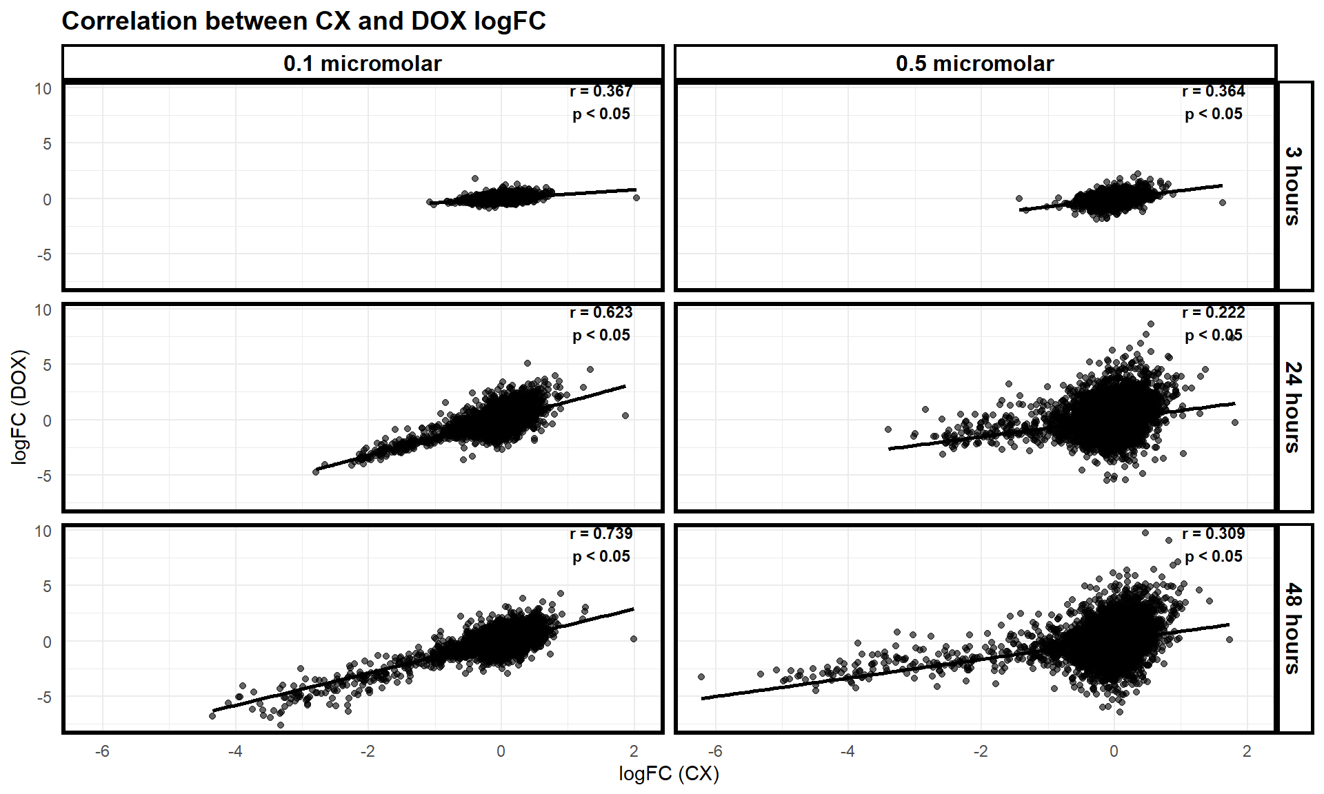
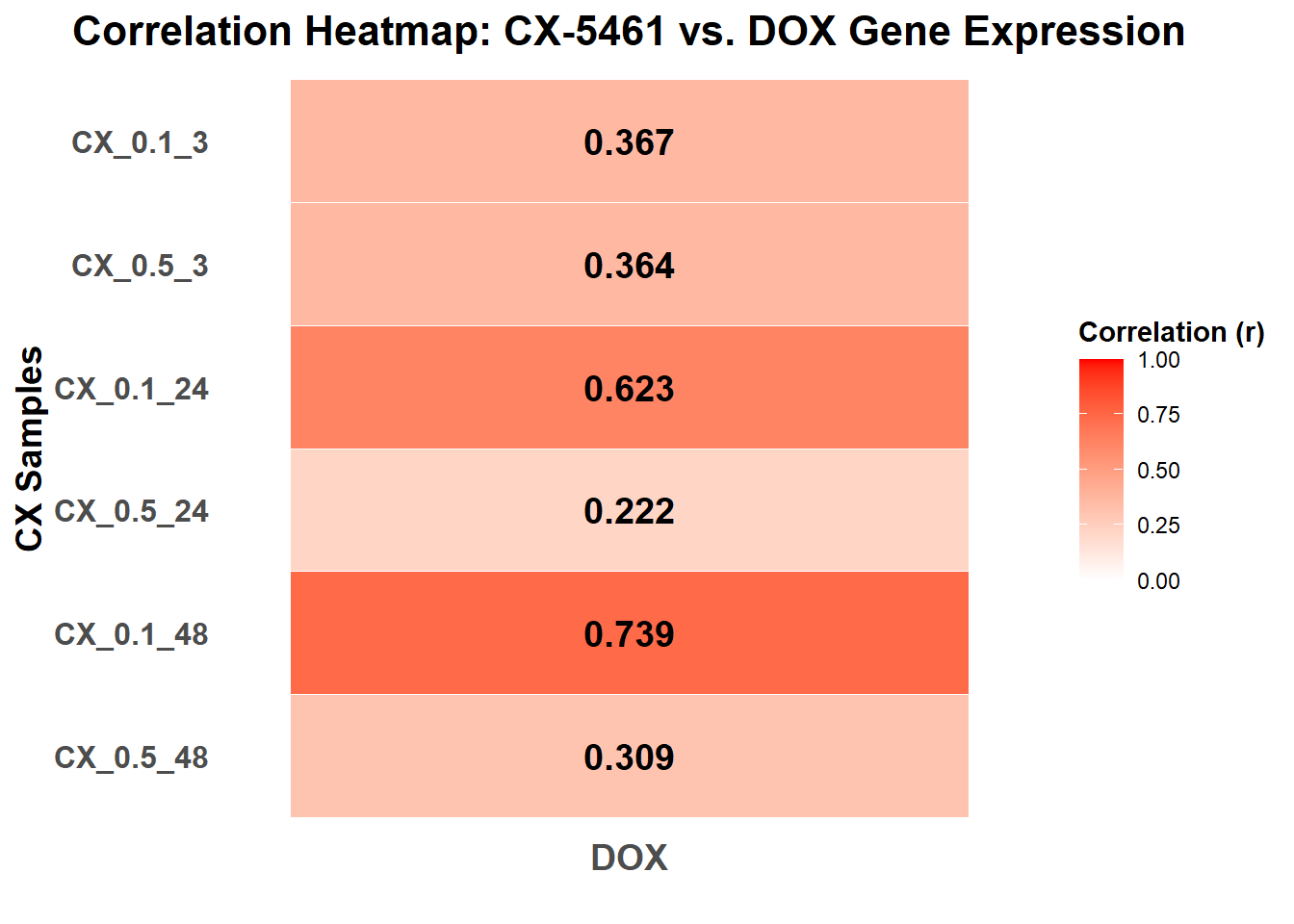
📌 Correlation Heatmap
# Load necessary libraries
library(ggplot2)
library(reshape2)
library(dplyr)

# Define dataset pairs for correlation analysis
dataset_pairs <- list(
  list("CX_0.1_3", CX_0.1_3, "DOX_0.1_3", DOX_0.1_3),
  list("CX_0.1_24", CX_0.1_24, "DOX_0.1_24", DOX_0.1_24),
  list("CX_0.1_48", CX_0.1_48, "DOX_0.1_48", DOX_0.1_48),
  list("CX_0.5_3", CX_0.5_3, "DOX_0.5_3", DOX_0.5_3),
  list("CX_0.5_24", CX_0.5_24, "DOX_0.5_24", DOX_0.5_24),
  list("CX_0.5_48", CX_0.5_48, "DOX_0.5_48", DOX_0.5_48)
)

# Create an empty data frame to store correlations
correlation_data <- data.frame(CX_Sample = character(), Correlation = numeric())

# Compute correlations for each CX vs. DOX dataset pair
for (pair in dataset_pairs) {
  cx_name <- pair[[1]]
  cx_data <- pair[[2]]
  dox_name <- pair[[3]]
  dox_data <- pair[[4]]

  # Merge datasets on Entrez_ID
  merged_data <- merge(cx_data, dox_data, by = "Entrez_ID", suffixes = c("_CX", "_DOX"))

  # Compute Pearson correlation
  r_value <- cor(merged_data$logFC_CX, merged_data$logFC_DOX, method = "pearson", use = "complete.obs")

  # Clamp between 0 and 1
  r_value <- max(0, min(1, r_value))

  # Store the result
  correlation_data <- rbind(correlation_data, data.frame(CX_Sample = cx_name, Correlation = r_value))
}

# Add a single column category for labeling
correlation_data$Comparison <- "DOX"

# Convert to long format for ggplot
heatmap_data_long <- melt(correlation_data, id.vars = c("CX_Sample", "Comparison"))

# Ensure the Y-axis follows the correct ordering (CX samples top to bottom)
heatmap_data_long$CX_Sample <- factor(heatmap_data_long$CX_Sample, levels = rev(c(
  "CX_0.1_3", "CX_0.5_3",
  "CX_0.1_24", "CX_0.5_24",
  "CX_0.1_48", "CX_0.5_48"
)))

# Create the CX vs. DOX correlation heatmap (0 to 1, white to red)
ggplot(heatmap_data_long, aes(x = Comparison, y = CX_Sample, fill = value)) +
  geom_tile(color = "white") +
  scale_fill_gradient(low = "white", high = "red", limits = c(0, 1)) +
  geom_text(aes(label = round(value, 3)), color = "black", size = 5, fontface = "bold") +
  labs(
    x = "", y = "CX Samples", fill = "Correlation (r)",
    title = "Correlation Heatmap: CX-5461 vs. DOX Gene Expression"
  ) +
  theme_minimal() +
  theme(
    axis.text.x = element_text(face = "bold", size = 14),
    axis.text.y = element_text(face = "bold", size = 12),
    axis.title.y = element_text(face = "bold", size = 14),
    plot.title = element_text(face = "bold", hjust = 0.5, size = 16),
    legend.title = element_text(face = "bold"),
    panel.grid = element_blank()
  )
sessionInfo()R version 4.3.0 (2023-04-21 ucrt)
Platform: x86_64-w64-mingw32/x64 (64-bit)
Running under: Windows 11 x64 (build 26100)
Matrix products: default
locale:
[1] LC_COLLATE=English_United States.utf8
[2] LC_CTYPE=English_United States.utf8
[3] LC_MONETARY=English_United States.utf8
[4] LC_NUMERIC=C
[5] LC_TIME=English_United States.utf8
time zone: America/Chicago
tzcode source: internal
attached base packages:
[1] stats graphics grDevices utils datasets methods base
other attached packages:
[1] reshape2_1.4.4 ggplot2_3.5.1 dplyr_1.1.4 workflowr_1.7.1
loaded via a namespace (and not attached):
[1] sass_0.4.9 generics_0.1.3 stringi_1.8.3 lattice_0.22-5
[5] digest_0.6.34 magrittr_2.0.3 evaluate_1.0.3 grid_4.3.0
[9] fastmap_1.1.1 plyr_1.8.9 rprojroot_2.0.4 jsonlite_1.8.9
[13] Matrix_1.6-1.1 processx_3.8.5 whisker_0.4.1 ps_1.8.1
[17] promises_1.3.0 httr_1.4.7 mgcv_1.9-1 scales_1.3.0
[21] jquerylib_0.1.4 cli_3.6.1 rlang_1.1.3 munsell_0.5.1
[25] splines_4.3.0 withr_3.0.2 cachem_1.0.8 yaml_2.3.10
[29] tools_4.3.0 colorspace_2.1-0 httpuv_1.6.15 vctrs_0.6.5
[33] R6_2.5.1 lifecycle_1.0.4 git2r_0.35.0 stringr_1.5.1
[37] fs_1.6.3 pkgconfig_2.0.3 callr_3.7.6 pillar_1.10.1
[41] bslib_0.8.0 later_1.3.2 gtable_0.3.6 glue_1.7.0
[45] Rcpp_1.0.12 xfun_0.50 tibble_3.2.1 tidyselect_1.2.1
[49] rstudioapi_0.17.1 knitr_1.49 farver_2.1.2 htmltools_0.5.8.1
[53] nlme_3.1-166 rmarkdown_2.29 labeling_0.4.3 compiler_4.3.0
[57] getPass_0.2-4